
1 Anidolic optics and Monge Ampère type equations
In anidolic optics, or non-imaging optics, one studies the design of devices that transfer light energy between a source and a target. The general problem is to design the shape of a mirror (or a lens) that reflects (or refracts) the light emitted from a given source towards a target whose geometry and intensity distributions are prescribed (see Figures 1 and 2). Applications of anidolic optics include the design of solar ovens, public lighting, car headlights, and more generally the optimization of the use of light energy and the reduction of light pollution.
Near-field and far-field light sources
There exists many different problems in anidolic optics, depending for instance on the geometry of the light source, the type of optical component, and the target to be illuminated. These problems are distinguished in particular by the spatial position of the target illumination. A problem is called near-field when the target is located within a finite distance, i.e., when one wishes to illuminate an area of space such as a screen. In Figures 1 and 2, the target illumination is on a wall, making the problem near-field. Most of the illustrations in this article correspond near-field targets. However, we will first consider the far-field case, which is mathematically simpler, and in which the target lies “at infinity”, in the space of directions. In practice, this means that when light is reflected or refracted from a point of the optical component, we can forget the spatial position of the reflected or refracted ray, keeping only its direction, which can then be encoded by a unit vector. Note that if the near-field target illumination is far away from the optical component, each point of the target almost corresponds to a direction, so that the far-field problem is a good approximation of the near-field one in this situation. We will see in Section 4.2 that one can solve a problem involving a near-field target by iteratively solving problems with far-field targets.
We will first present two far-field mirror problems in their continuous form, as illustrated in Figure 1. Then, we will explain how these continuous problems can be approached by discrete problems, following the so-called supporting quadric method introduced by Luis Caffarelli and Vladimir Oliker. This method can be traced back to work of Hermann Minkowski and Aleksandr Aleksandrov in convex geometry.

1.1 Mirror for a point light source
In this first problem, light is emitted from a point , which we assume to be located at the origin of the space . The intensity of the light source is modeled by a probability density on the sphere of directions . Let denote the support of the measure . For example, if the light is emitted in a solid cone, then is a disc on the sphere. The quantity of light emanating from a measurable set of directions is given by . For the far-field problem, the target is described by a probability measure on the sphere of directions , which then represents the directions “at infinity”, i.e., after reflection. Let denote the support of the measure .
The inverse problem considered here consists in constructing the surface of a mirror which will transport the intensity of the light source to the desired light distribution at infinity using Snell’s law of reflection. For example, if the target measure is a Dirac mass , meaning that we want to reflect all the light in a single direction , then the shape of the mirror is given by a paraboloid of revolution.
Let denote the Euclidean scalar product on . An incident ray is reflected by a surface in the direction , where is the unit vector normal to the surface at the point touched by the direction and oriented so that . The surface solves the inverse mirror problem if transports the source measure to the target measure , in the sense that for any measurable subset of the sphere one has
Note that the preservation of overall light quantity was already ensured by having chosen probability measures, i.e., . Now assume that and are absolutely continuous measures with respect to the area measure on the sphere. Let and , where and are the densities of and respectively. The previous equation then reads
Suppose furthermore that the densities et are continuous and that is a diffeomorphism from to . By the change of variable , the last equation is then equivalent to for any .
Since the mirror reflects rays emitted from the origin, we will assume that the surface is radially parametrized by , where is a positive function that must be determined. The unit normal to the surface at the point and the direction of the reflected ray can both be expressed as a function of and of the gradient :
This allows us to formulate the problem as a system of partial differential equations, i.e., the problem of finding a positive function of class which satisfies
The first line of equation (Mir-Ponc-C) involves the determinant of a quantity which depends on the second derivatives of . This equation belongs to the family of Monge–Ampère equations. Note that the requirement that is a diffeomorphism is non-standard and difficult to handle. In practice, it is replaced by a condition on which is akin to convexity, and by the so-called second boundary condition . These two conditions ensure the ellipticity of the problem. Caffarelli and Oliker proved in 1994 [1 L. Caffarelli and V. Oliker, Weak solutions of one inverse problem in geometric optics. Journal of Mathematical Sciences154, 39–49 (2008) ] the existence of weak solutions to this equation, i.e., the existence of a locally Lipschitz function such that the application defined by the last two lines of (Mir-Ponc-C) satisfies (1). The existence of regular solutions to the problem (Mir-Ponc-C) is due to Wang and Guan [6 X.-J. Wang, On the design of a reflector antenna. Inverse Problems12, 351–375 (1996) , 2 P. Guan and X.-J. Wang, On a monge-ampere equation arising in geometric optics. J. Differential Geom48, 205–223 (1998) ].
1.2 Mirror for a collimated light source
We now present a second inverse problem arising in anidolic optics. This time the light source is collimated, which means that all the rays of light emitted by the source are parallel. We furthermore assume that they are positively collinear to the vertical vector and emitted from a domain of the horizontal plane . For convenience, we will identify and . We assume that the surface of the optical component is smooth and parametrized by a height function . The intensity of the light source is modeled by a probability measure on . As in the previous case, the intensity of the target illumination is modeled by a probability measure on the sphere of directions at infinity. At each point of the optical component, the gradient encodes the direction of the normal to the surface and we denote by the direction of the ray reflected by Snell’s law. The reflector defined by solves the inverse mirror problem between and if for any measurable set one has
Let us introduce the measure defined by , which is supported on . We assume that and are absolutely continuous with respect to the Lebesgue measure, with continuous densities and , and that is a diffeomorphism on its image. Then, with the change of variable , the inverse mirror problem for a collimated source can also be phrased as a partial differential equation:
We finally note that if is smooth and strongly convex (or strongly concave), the application is a diffeomorphism on its image.
1.3 Lenses
The construction of lenses that transform a light source into a target illumination prescribed at infinity are similar and are also described by Monge–Ampère type equations. As with mirrors, when the light is emitted from a point, the equation to be solved is on the sphere and when the light source is collimated, it is on the plane. In these problems, the light source passes through the surface of one side of the lens, either flat or spherical, and the aim is to construct the surface of the other side of the lens such that it refracts the light onto a prescribed target illumination at infinity. We do not detail the modelling of these problems here, but we will show results with lenses at the end.
2 Geometric discretization of Monge–Ampère equations
The two inverse problems in anidolic optics described in the previous section each involve two sets and , on which we have two probability measures and respectively, representing the light source and the desired target illumination. We saw that when these measures are absolutely continuous, the problems of construction of optical components correspond to partial differential equations of Monge–Ampère type.
The most direct method to solve a partial differential equation numerically is to approximate the domain with a discrete grid and to replace the partial derivatives with differences of the values of the function at the points of the grid divided by the grid step. In the case of Monge–Ampère equations, the application of these methods is made difficult by the non-linearity of the Monge–Ampère operator and by the diffeomorphism condition. We refer to the work of Adam Oberman, Brittany Froese, Jean-David Benamou and Jean-Marie Mirebeau for this line of research.
In recent years, alternative methods, called semi-discrete methods, have been used to discretize and numerically solve Monge–Ampère type equations arising from optimal transport. In order to apply this method, one assumes that one of the two measures or is absolutely continuous, while the other is finitely supported. Here we assume that has a density on the space and that is a discrete measure on the space , i.e., where is the Dirac mass in .
In this section, we describe the semi-discrete variant of the two far-field mirror problems seen in the previous section, leaving aside the problem of convergence of the solutions to the discrete problems towards those to the continuous problems. These constructions give rise to equations which can naturally be seen as discrete Monge–Ampère equations. We also propose an economic interpretation by addressing the bakeries problem.
2.1 Mirror for a point light source
Let us go back to the problem of constructing mirrors that transform the light emitted by a point light source (see Section 1.1). As in the previous section, the light source is modeled by a continuous probability density on the sphere of directions , whose support corresponds to the set of directions in which light is emitted. This time we assume that the desired target illumination is described by a probability measure supported on a set of distinct directions. The problem is still to find the mirror surface that will reflect the measure onto the measure under Snell’s law, but this time the target measure is discrete.
Mirror composed of paraboloid pieces
We use the method of supporting paraboloids proposed by Caffarelli and Oliker in 1994 [1 L. Caffarelli and V. Oliker, Weak solutions of one inverse problem in geometric optics. Journal of Mathematical Sciences154, 39–49 (2008) ], which was originally developed to show the existence of weak solutions in the case where both measures are absolutely continuous. Caffarelli and Oliker’s idea is based on a well-known property of paraboloids of revolution: a paraboloid of revolution with focal point and direction reflects any ray coming from point to the direction . It is thus natural to seek to construct a mirror whose surface is composed of pieces of paraboloids, each paraboloid illuminating a direction .
More precisely, we take and denote by the solid (i.e. filled) paraboloid of direction , with focal point at the origin and focal distance . This means that is the distance between and the paraboloid’s closest point to . We define by the surface bordering the intersection of the solid paraboloids :
For each we denote by the set of rays emitted by the light source and reflected by Snell’s law in the direction . This set is called the -th visibility cell of the mirror . By construction, it corresponds to the radial projection of onto the sphere (see Figure 2.1).
A simple calculation shows that the intersection of two confocal paraboloids and is included in a plane curve. Projecting radially onto the unit sphere, this implies that the intersection of two visibility cells is included in a curve on the sphere. We deduce that the set of visibility cells forms a partition of the sphere , up to a set of measure zero.
The paraboloid of revolution can be parametrized radially by the function , where . We deduce that belongs to the visibility cell if and only if the distance is smaller than the distances for . Composing with the logarithm to linearize the expression in , we obtain an explicit expression for the visibility cells
where .
By construction, each ray emitted by the point source and belonging to the cell hits the mirror at a point which belongs to the paraboloid and which is reflected in the direction . The quantity of light received in the direction is therefore exactly the quantity of light emanating from the visibility cell , i.e., . The desired quantity of light in the direction is . The equation to be solved is therefore for any . Moreover, note that a paraboloid of revolution is only determined by its focal point, its direction and its focal distance. The free parameter remaining for each paraboloid is the focal distance .

Formulation of the problem
The semi-discrete far-field mirror problem for a point source can be formulated as the problem of finding focal distances that satisfy
where and where
We will see in Section 3 how to solve such systems of equations. Note that if is a vector of focal distances solving the mirror problem for a point-like source, then the surface of the mirror is parametrized by
In the numerical experiments, we assume that the target illumination is included in the half-sphere , that the support of is included in the half-sphere , and that the mirror is parametrized above the domain .
Remark 2.1. The mirror surface is by construction the boundary of a convex set, i.e., the intersection of the solid paraboloids . It is also possible to construct a mirror contained in the boundary of the union of solid paraboloids rather than an intersection. This produces mirrors that are somewhat less interesting in practice, as they are neither convex nor concave.
2.2 Mirror for a collimated light source
Let us now consider the mirror problem for a collimated light source, already seen in Section 1.2. As before, the probability measure modelling the light source has a density with respect to the Lebesgue measure on the plane. However the probability measure modelling the target illumination intensity is discrete , supported on a finite set of distinct directions. The problem is, again, to find the surface of a mirror which reflects the measure to the measure .
Mirror with planar faces
We choose to construct the mirror surface as the graph of affine height functions of the form (see Figure 2.2). The vector is chosen so that the plane reflects vertical rays, i.e., with direction , into the direction . We need to determine the heights of those planes. Given a family of heights , we define the -th visibility cell as

By construction, for each , any vertical ray emitted from a point hits the mirror at a height and is reflected in the direction . Thus, the amount of light reflected in the direction is equal to .
Formulation of the problem
Solving the semi-discrete far-field mirror problem for a collimated light source amounts to finding the heights that satisfies
where and
A solution of the equation (Mir-Colli-SD) induces a parametrization of the convex mirror that reflects onto :
In practice, we only consider the part of the mirror located above the domain .
Remark 2.2. The function being the maximum of affine functions, it is convex. The optical component which is parametrized by the graph of this application is also convex. Note that one could have the same construction by replacing the in the formula by a . This would result in a concave function and a concave mirror.
Remark 2.3. Problem (Mir-Colli-SD) is very similar (but not equivalent) to Minkowski’s problem in convex geometry which is also an inverse problem. Given a set of unit vectors and real numbers , this problem consists in building a convex polyhedron whose -th facet has normal and area – which is possible only under some assumptions on the directions and areas. We also note that Oliker, who was the first to introduce semi-discrete methods for the numerical resolution of Monge–Ampère equations, was a doctoral student of the famous geometer Aleksandrov who is known (among other) for introducing and studying the “continuous” formulation of Minkowski’s problem.

2.3 The bakeries problem
We now present an economic analogy which leads to an equation having the same structure as in the two optical problems presented above. We assume that represents a city whose population density is described by a probability density , that the finite set represents the locations of the city’s bakeries and that represents the quantity of bread available in bakery . Customers living at a location in naturally will look for the bakery minimizing the cost of walking from to , denoted . This leads to a decomposition of the city space into Voronoi cells,
The number of customers going to a bakery is equal to the integral of the density over . Suppose that a bakery receives too many customers in comparison to its bread’s production capacity – this could be the case in Figure 6 for the downtown bakery where the population density is high. This means we have , where we denote . The baker will then seek to increase the price of his bread. This will reduce the number of potential customers, but will increase the baker’s profit as long as he manages to sell all his stock. We write for the proportion of the population that the bakery is able to serve, and the price of the bread in the bakery . If we assume that the customers living at point make a compromise between walking cost and price of bread by minimizing the sum (), the city is then decomposed into Laguerre cells
Note that we do not necessarily have , and that it is even possible to have : indeed, if the bread is very expensive in a certain bakery, even people living next door may prefer going to a more distant one.
Problem formulation
The bakeries problem therefore boils down to finding a price vector such that each bakery sells all its stock of bread . This is described by the system of equations
This equation has exactly the same structure as (Mir-Ponc-SD) and (Mir-Colli-SD). We will see in the next section how to solve this class of equations.
3 Numerical resolution
The discrete problems mentioned in the previous section all show the same structure; our focus will now be on their numerical resolution. We start by introducing the semi-discrete Monge–Ampère equation, and show that its solution is equivalent to finding the maximum of a concave function. Subsequently, we present a Newton method that allows us to solve these equations efficiently.
3.1 Semi-discrete Monge–Ampère equation
Let be a compact subset of the space or of the sphere , let , and let be a cost function. The Laguerre cell (which corresponds to a visibility cell in optics) associated with a family of real numbers is given by
Suppose that the cost function satisfies the Twist condition
which ensures that the Laguerre cells form a partition of the domain up to a negligible set.
Semi-discrete Monge–Ampère equation
Let be a probability measure on with density with respect to the area measure, and let be a probability measure on . In the following equation, the discrete probability measure is conflated with the vector . We are seeking satisfying
where the function is defined by
Remark 3.1. The visibility cells used in optics in (Mir-Ponc-SD) and (Mir-Colli-SD) are Laguerre cells, with
respectively. Equation (MA) is a reformulation of equations (Mir-Ponc-SD) and (Mir-Colli-SD). Note that the Laguerre cells are invariant under addition of a constant to , and that the solution of (MA) is therefore defined up to an additive constant. Optical problems have a similar invariance: for example, if a surface is a solution of the mirror problem for a point source, then so is for all .
3.2 Variational formulation
The following theorem shows that the function in the semi-discrete Monge–Ampère equation is the gradient of a concave function.
We assume that the cost function satisfies (Twist). Then the function defined by
is concave, of class and with gradient
As we will see in the next paragraph, the function is related to the Kantorovitch duality in optimal transport theory, and we will therefore call it the Kantorovitch functional. Moreover, since a concave function of class reaches its maximum exactly at its critical points, we obtain the following corollary:
Corollary 3.2. Under the assumptions of Theorem 3.1, a vector is a solution to equation (MA) if and only if is a maximizer of .
Since the function is invariant under addition of a constant, one can choose to work on the set of vectors whose coordinates sum to zero. It can be shown that the function is proper on , i.e., , which ensures that it reaches its maximum: the problem (MA) thus admits a solution.
3.3 Relation to optimal transport
The variational formulation of the Monge–Ampère equation, i.e., the search for a maximizer of the Kantorovitch functional, corresponds in fact to the dual of the Monge–Kantorovitch problem in optimal transport theory. We discuss this link in detail below in the semi-discrete case. The reader interested in the proofs may refer for instance to the book chapter [4 Q. Mérigot and B. Thibert, Optimal transport: Discretization and algorithms. In Handbook of Numerical Analysis, Geometric PDEs 22, Elsevier, 621–679 (2020) ].
Monge’s problem
The image of a probability measure on under a measurable application is the measure on defined by . If , we say that transports to . Since the set is finite, we have . Monge’s optimal transport problem consists in finding a transport map that transports to and that minimizes the total cost . If the cost function satisfies the Twist condition, Brenier and Gangbo–McCann, relying on Kantorovich duality, proved the existence of a minimizer for this problem when the source is absolutely continuous. For example, one can state the following:
Suppose that satisfies the condition (Twist) and that is absolutely continuous. Then
If moreover is a maximizer of , then the function defined -a.e. by realizes the minimum in Monge’s problem.
Remark 3.2. Not all Monge–Ampère equations derive from an optimal transport problem and not all of them admit a variational formulations. These two strong properties come in fact from the very particular structure of Laguerre cells, which follows from the functions being affine.
We saw that the far-field optics problems presented in Section 2 possess this structure. On the other hand, if we consider the mirror construction problems for a target illumination in the near-field (i.e., we are illuminating points in and not directions at infinity), we still have semi-discrete Monge–Ampère equations to solve, but the Laguerre cells are of the form
where the function is nonlinear in . These equations do not derive from the optimal transport problem and in fact do not admit a variational formulation. They are called prescribed Jacobian equations by Trudinger, and are the subject of recent research both in analysis and in more applied fields (optics, economics).
3.4 Laguerre cells and derivatives
Before applying Newton’s method to solve the equation , we need to show that the function is of class (or equivalently that is of class ), calculate its partial derivatives and study the (strict) concavity of . To do this, we need a genericity assumption which is somewhat technical, but which is natural and not restrictive in practice. In the optical cases mentioned in this paper, this assumption is satisfied if the intersection of three distinct Laguerre cells is finite and if the intersection of two Laguerre cells with the boundary of is also finite. For more details, the reader may refer to the book chapter [4 Q. Mérigot and B. Thibert, Optimal transport: Discretization and algorithms. In Handbook of Numerical Analysis, Geometric PDEs 22, Elsevier, 621–679 (2020) ].
Suppose that the cost satisfies (Twist), that is generic (see above), and is continuous. Then the application is of class and
where .
The formula for the partial derivatives of has a geometric interpretation. In the following two figures, which are obtained for the cost on , we explain why the formula for partial derivatives involves integrals over the interfaces between Laguerre cells and how the singularities of may occur depending on the geometry of the points .
Figure 3.4 illustrates that the partial derivative is an integral over the interface : the value is an integral over the Laguerre cell (in grey on the left); we increase the value by considering ; the rate of increase is proportional to an integral over the symmetric difference between two Laguerre cells (in grey in the middle); passing to the limit we obtain an integral over the green segment . The signs that occurs in the formula for the partial derivatives can also be interpreted with the bakeries metaphor: when the price of bread increases, the number of customers of the bakery decreases (i.e., the Laguerre cell shrinks) and the number of customers for the other bakeries increases, so that and for .
In Figure 3.4, the genericity condition is not satisfied because , and are aligned, and there exists for which is a line segment. The partial derivative is an integral on the (green) segment . If we simultaneously decrease and by the same amount, we can see that the segment varies continuously and then suddenly becomes empty when the cell gets empty (bottom right of Figure 3.4). Thus, is not continuous. Newton’s method requires a certain regularity, and we will see below that it converges under the above genericity assumptions.


To establish the convergence of Newton’s method, we also need to study the concavity of the Kantorovitch functional , or equivalently the monotonicity of its gradient . The functions and are invariant by addition of a constant vector (i.e., ), which can be seen in the definition of Laguerre cells. Thus, we can only hope to establish strong concavity of in the directions orthogonal to constant vectors, i.e., belonging to the set
Another reason for the lack of strong concavity of is that if is very large, then is empty and remains empty in a neighborhood of . In this case, is constant equal to zero, and the Hessian matrix has a row of zeros. We can therefore hope to establish strong concavity only if belongs to the set
The next theorem shows, in a nutshell, that these are the only two obstructions to strong concavity.
We assume the hypotheses of the previous theorem hold. If the set is connected, the function is locally strongly concave on in the direction :
Remark 3.3 (Uniqueness). We saw above that the function has a maximum, and thus equation (MA) has a solution. The previous theorem implies that this maximum is unique if we impose that , i.e., has zero average, since a strictly concave function admits at most one local maximum.
We will see in the next paragraph how these results of regularity and monotonicity allow us to iteratively construct a sequence converging to the unique zero-average satisfying .
3.5 Newton’s method
Newton’s method in 1D
We begin by recalling Newton’s method for solving the equation , where is a real function. Newton’s method starts from and constructs the sequence by induction. If we assume that is of class and that there exists such that and , then one can show, using Taylor–Lagrange formulas, that for sufficiently close to , the sequence converges to . The convergence is then said to be local. Thus, under a regularity hypothesis () and monotonicity ( has constant sign in a neighborhood of ), Newton’s method converges locally.
Newton’s method (local)
Assume that we are given a zero-average vector such that the mass of all Laguerre cells is strictly positive:
We define in the following way: we start by calculating the Newton direction , i.e., the vector satisfying
which exists and is unique by according to Theorem 3.5. The second equation enables us to overcome the invariance of and thus the non-invertibility of . We then define . As in the 1D case, it can be shown that the method converges locally: if is chosen close enough to the solution, then the sequence converges to .
Globally convergent Newton’s method
However, the condition is close to the solution is impossible to fulfill in practice. Fortunately, a very simple modification of the method allows to ensure a global convergence, allowing us to drop this closeness assumption. To do this, one must construct in such a way that the kernel of the Jacobian remains equal to constant vectors, so that the system defining the direction admits a unique solution. For this purpose, we define the step as the largest real of the form (with ) such that satisfies
Finally, we define .
By using the regularity and concavity results on , the step can be bounded from below, thus ensuring the convergence of the sequence constructed above to a solution of the optimal transport problem [4 Q. Mérigot and B. Thibert, Optimal transport: Discretization and algorithms. In Handbook of Numerical Analysis, Geometric PDEs 22, Elsevier, 621–679 (2020) ]:
Under the assumptions of Theorem 3.5, there exists such that
In particular, the sequence converges to the unique solution of (MA) satisfying .
Remark 3.4 (Quadratic convergence). The above theorem shows that the convergence of Newton’s method is globally exponential. This convergence is actually called linear convergence in optimization. When the cost satisfies the Ma–Trudinger–Wang (MTW) condition that appears in the theory of optimal transport regularity, and the density is Lipschitz, then the convergence is even locally quadratic [3 J. Kitagawa, Q. Mérigot and B. Thibert, Convergence of a Newton algorithm for semi-discrete optimal transport. Journal of the European Mathematical Society (2019) ]: for sufficiently large , we have
In practice, the convergence is very fast and the basin where quadratic convergence occurs seems to be quite large. This last observation is empirical, and not mathematically explained yet. In Figure 9, is the large white square and is a set of points in the lower left corner and . With points, after three iterations the error is already of order . Even difficult examples of size in dimension can be solved to high numerical precision with less than 20 iterations!
4 Applications to anidolic optics
In this section we present the adaptation of semi-discrete methods to the practical resolution of inverse problems in optics. These results were obtained in the PhD thesis of Jocelyn Meyron and the images are taken from the article [5 J. Meyron, Q. Mérigot and B. Thibert, Light in power: A general and parameter-free algorithm for caustic design. In SIGGRAPH Asia 2018 Technical Papers, ACM Transaction on Graphics, p. 224 (2018) ].

4.1 Far-field problems
We saw in Section 2 that in several far-field problems, i.e., when the target illumination is at infinity, solving the Monge–Ampère equation (MA) allows us to construct an optical component. This involves modelling mirrors or lenses, with a point or collimated light source, and in each case there are two components that may be produced (one of which is convex), so that in all we have formulated eight different near-field optical problems.
The main difficulty in implementing Newton’s algorithm to solve (MA) lies in the evaluation of the function and its differential at point , and more precisely in the calculation of the set of Laguerre cells . For cells from non-imaging optics problems, also called visibility cells, it is possible to perform this calculation in almost linear time in the number of Dirac masses. Take for example the mirror problem for a point source. The visibility cells are obtained by projecting radially onto the sphere an intersection of “solid” confocal paraboloids, and we have already seen that the intersection of two confocal paraboloids is included in a plane. Another simple calculation shows that the radial projection of such an intersection is also included in a (different) plane. This shows that the visibility cells are separated by hyperplanes. In fact, it can be shown that there exists a partition of into convex polyhedra – called a power diagram in computational geometry – such that each visibility cell is of the form (Figure 4.1). A similar property holds for each of the eight problems. The point of this reformulation is that there are powerful libraries – for example Cgal or Geogram – that allow us to compute power diagrams in dimensions and , and thus also the Laguerre cells associated with the optics problems. It is therefore possible to implement the damped Newton algorithm, and to use it to construct – numerically and even physically – mirrors and lenses for far-field targets in anidolic optics.

4.2 Near-field problems
It is also possible to deal with more realistic target illuminations in the near-field – i.e., when illuminating points at a finite distance rather than directions – with an iterative method that solves a far-field solution at each step [5 J. Meyron, Q. Mérigot and B. Thibert, Light in power: A general and parameter-free algorithm for caustic design. In SIGGRAPH Asia 2018 Technical Papers, ACM Transaction on Graphics, p. 224 (2018) ]. The convergence is very fast, requiring only a few iterations, as illustrated in Figure 4.2.
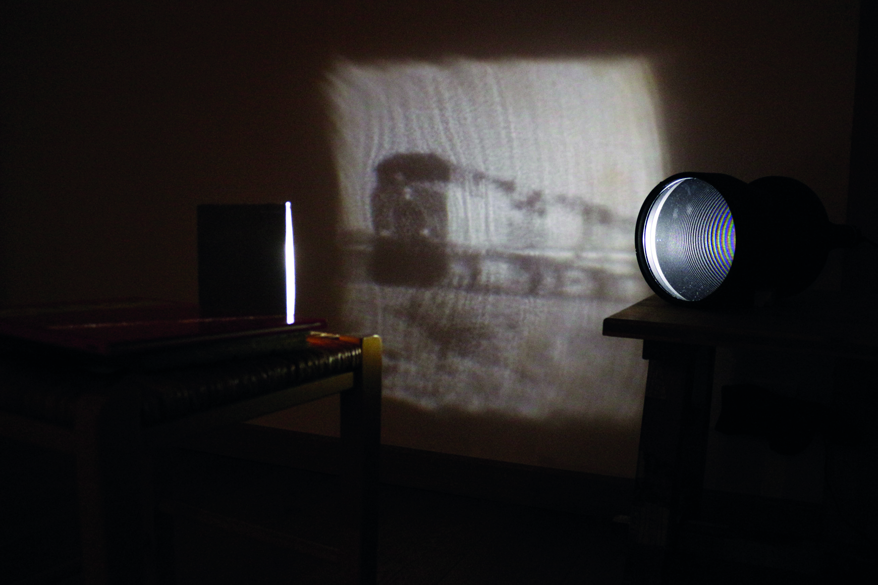
In all the experiments presented below, the light source is assumed to be uniform, so that the light source has a constant density on its support. The reflection or refraction of this light on a wall is simulated in the computer by the physically realistic rendering software LuxRender.
Generic method
The different problems of anidolic optics having the same structure (point or collimated light sources, mirrors or lenses, convex or concave components, near-field or far-field), it is possible to solve them in a unified, precise and automatic manner with the same


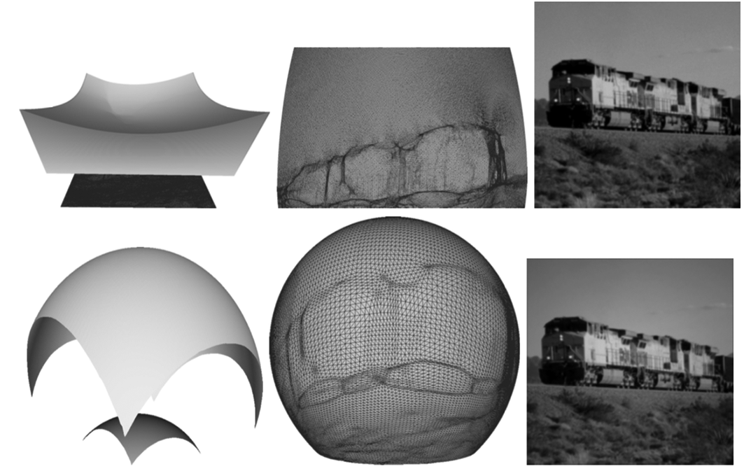
algorithm (Figures 4.2, 4.2 and 4.2). In Figures 4.2 and 4.2, the visibility cells on the sphere or plane are shown on the left, above which is the surface of the optical component. Each surface is represented in the computer by a mesh (a set of triangles) which is shown in the middle. The simulation of the reflected or reflacted light with LuxRender is on the left.
Convexity/concavity of the components
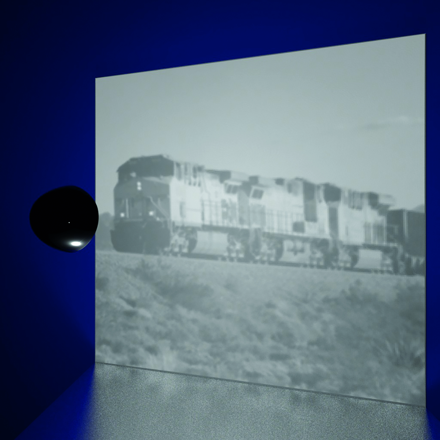
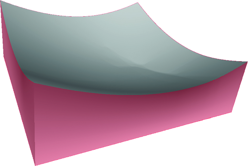
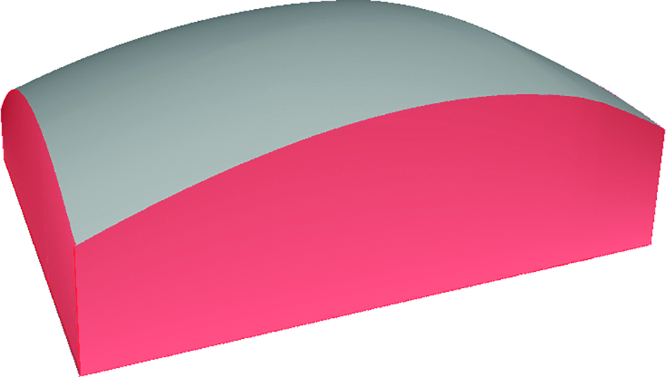
Some applications require the construction of optical components with convexity properties. This is the case in the automotive industry for the construction of mirrors and/or lenses. The reason for this is both practical, as it is easier to build a convex component, and aesthetic. In the case of collimated light sources, mirrors or lenses can always be convex or concave, as can be seen in Figure 4.2.
Singularity of solutions
The optical components are by construction objects with only a regularity. Indeed, they are surfaces composed of pieces of planes, paraboloids or ellipsoids (in the case of a mirror for a point light source) which are joined together in a manner that is continuous but not . However, as the discretization of the target illumination becomes finer and finer, the surface tends towards an object that has greater regularity. In Figure 4.2, we observe a regularity, except at points on the surface that correspond to black areas in

the target image. Intuitively, the lack of regularity comes from the fact that the light must avoid the black areas, which results in a jump in the vector field normal to the surface.
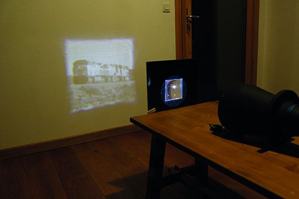
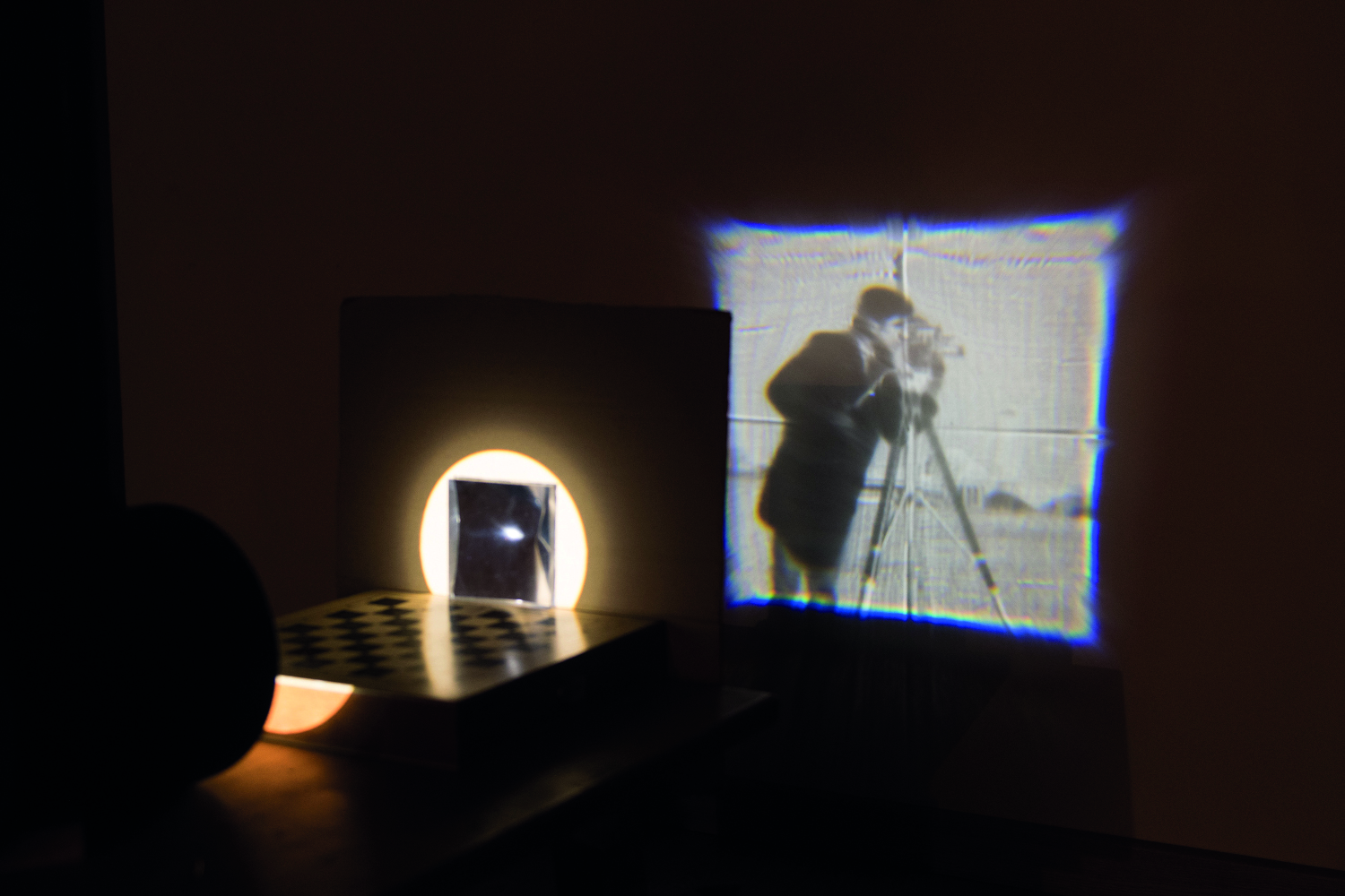
Pillows
The inner part of a car headlamp is typically made up of “pillows”, i.e., several small components. Each patch is intended to illuminate a fairly wide range of directions, and the lights sent out by each pillow overlap. This ensures a certain robustness in the lighting. If for instance a bird flies past the headlights, not too close, it does not obstruct all the light and the road remains fully illuminated. In Figure 4.2, the target illumination for each pillows is the cameraman’s image. When the calculations are done in the far-field, i.e., when illuminating directions, the images are superimposed, but with an offset due to the size of the pillows. To obtain a clear image, it is necessary to make the calculations in the near-field, so as to illuminate exactly the desired points. Note that the target is always illuminated even if an obstacle, for example a red monkey head, is placed in front of some of the pillows.
Colored target illumination
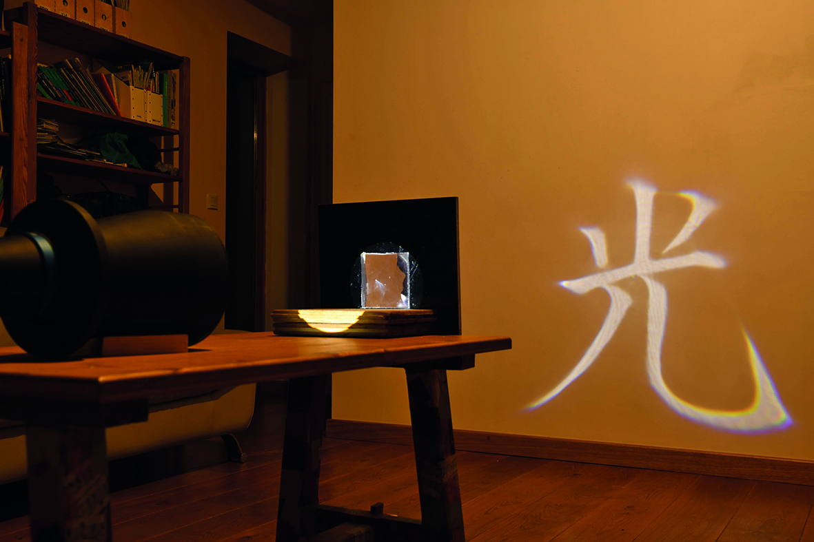
Similarly, solving the near-field problem makes it possible to illuminate a target in color. Indeed, one can build an optical component for each channel (red, green and blue). Then each of the three lights is sent to its associated component and the colors are added to the target to form a color image. This is done in Figure 4.2 with three lenses.
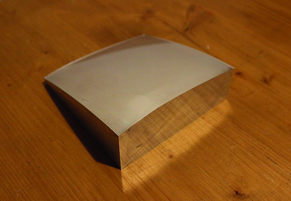
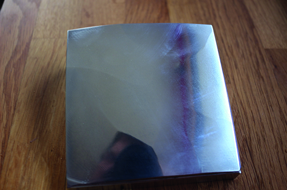
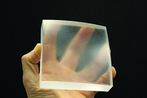
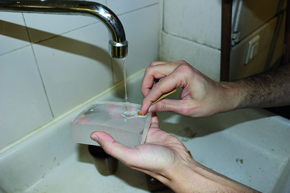
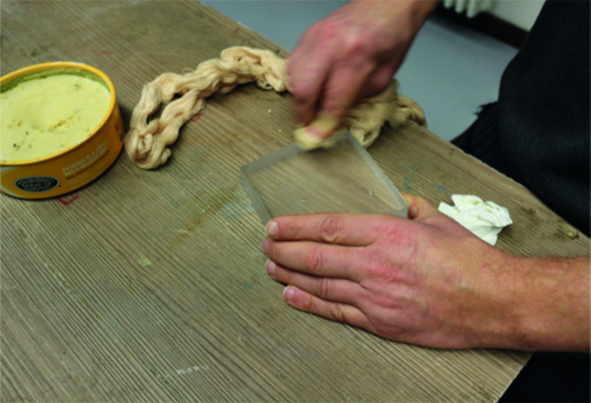
Construction of mirrors and lenses
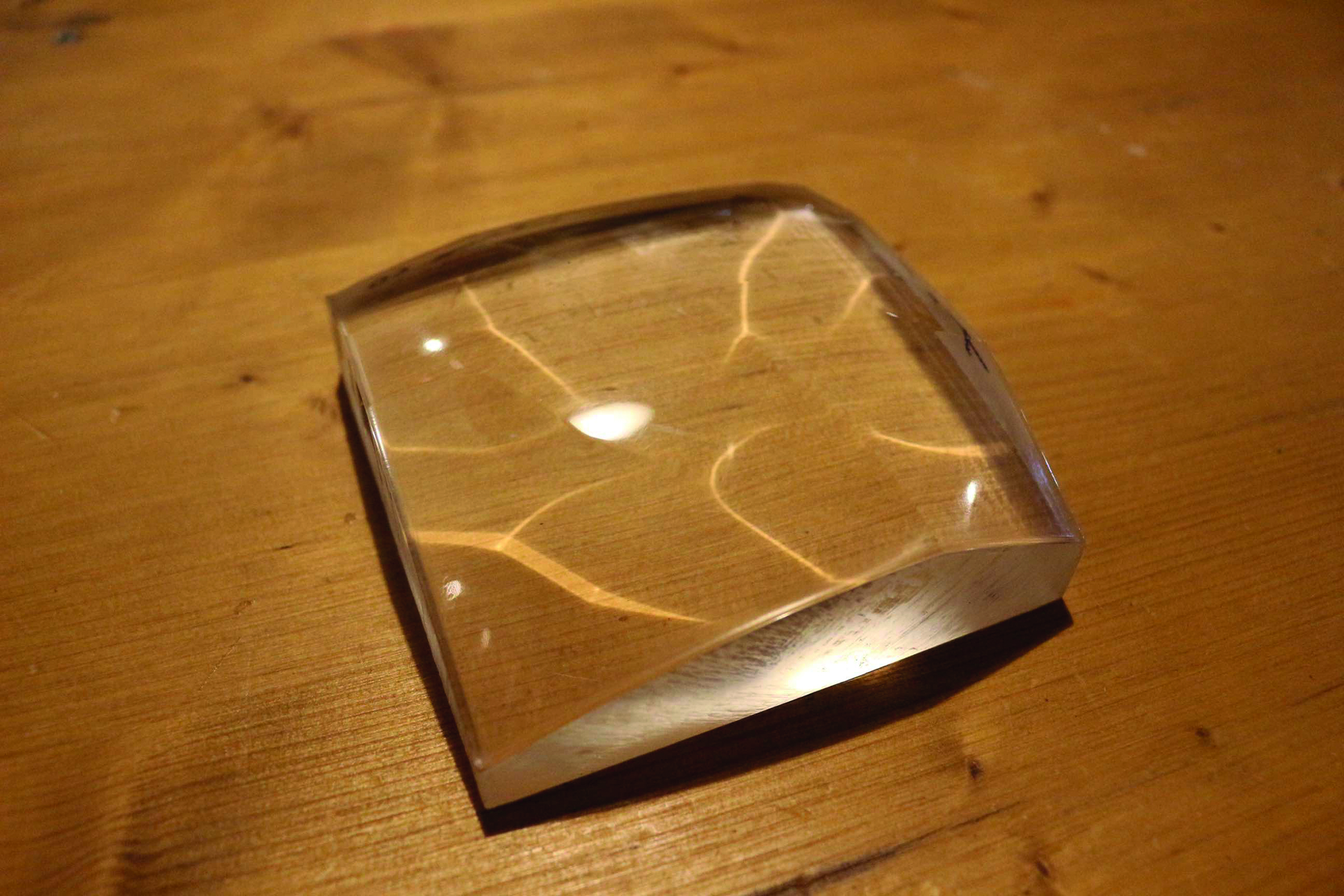
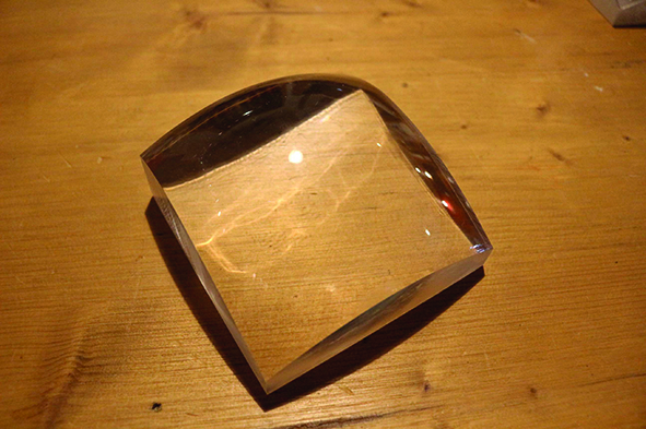
We also built optical components. The lenses and mirrors in Figures 4.2, 2 and 4.2 were milled by the GINOVA technology platform in Grenoble on a 3-axis CNC (computer numerical control) machine with 10 mm radius milling cutters. The path of the milling cutter creates irregularities on the optical components (Figure 4.2). Note that the convexity of the optical components allows the use of arbitrarily large milling radii, which reduces machining irregularities. In any case, it is necessary to grind under water and then polish the optical components (Figure 4.2). Of course, this affects the optical quality and tends to whiten the black areas in the target image.
Acknowledgements The authors thank Damien Gayet for his meticulous proofreading of the French version of this article, and for much good advice. The EMS Magazine thanks La Gazette des Mathématiciens for its authorisation to publish this text, which is an English translation of the original paper [La Gazette des Mathématiciens, Number 166, pp. 6–21, October 2020].


References
- L. Caffarelli and V. Oliker, Weak solutions of one inverse problem in geometric optics. Journal of Mathematical Sciences154, 39–49 (2008)
- P. Guan and X.-J. Wang, On a monge-ampere equation arising in geometric optics. J. Differential Geom48, 205–223 (1998)
- J. Kitagawa, Q. Mérigot and B. Thibert, Convergence of a Newton algorithm for semi-discrete optimal transport. Journal of the European Mathematical Society (2019)
- Q. Mérigot and B. Thibert, Optimal transport: Discretization and algorithms. In Handbook of Numerical Analysis, Geometric PDEs 22, Elsevier, 621–679 (2020)
- J. Meyron, Q. Mérigot and B. Thibert, Light in power: A general and parameter-free algorithm for caustic design. In SIGGRAPH Asia 2018 Technical Papers, ACM Transaction on Graphics, p. 224 (2018)
- X.-J. Wang, On the design of a reflector antenna. Inverse Problems12, 351–375 (1996)
Cite this article
Quentin Mérigot, Boris Thibert, Mirrors, lenses and Monge–Ampère equations. Eur. Math. Soc. Mag. 120 (2021), pp. 16–28
DOI 10.4171/MAG/21