Seeing the invisible: Digital holography

1 Introduction

Experimental sciences have traditionally been a source of challenging mathematical problems with a double edge: while mathematical theories are created, technology moves fast and industry develops. Imaging sciences provide a remarkable example. Typical imaging systems, such as radar [⁠28⁠ S. W. McCandless and C. R. Jackson, Principles of synthetic aperture radar. In SAR Marine Users Manual, NOAA (2004) ], magnetic resonance tomography, ultrasound, echography [⁠25⁠ A. Maier, S. Steidl, V. Christlein, J. Hornegger, Medical imaging systems: An introductory guide. Springer (2018) ], and seismic imaging [⁠34⁠ J. Tromp, Seismic wavefield imaging of Earth’s interior across scales. Nature Reviews Earth & Environment 1, 40–53 (2020) ], pose inverse scattering problems with a similar mathematical structure. In all of them, waves generated by a set of emitters interact with a medium under study and the wave field resulting from the interaction is recorded at a set of receivers [⁠10⁠ D. Colton and R. Kress, Inverse acoustic and electromagnetic scattering theory. Appl. Math. Sci. 93, Springer, Berlin (1992) ]. Different imaging systems resort to different types of waves and arrange emitters and receivers according to varied geometries. The nature of the employed waves depends on factors such as the size of the specimens under study, the contrast between components, and the damage caused to the sample during the imaging procedure. Knowing the emitted and recorded waves, we aim to infer the structure of the medium.

Approximating the solutions of inverse scattering problems is a challenging task because such problems are severely ill posed [⁠10⁠ D. Colton and R. Kress, Inverse acoustic and electromagnetic scattering theory. Appl. Math. Sci. 93, Springer, Berlin (1992) ]. Given arbitrary data, the problem under study may not admit a solution, the solution may not be unique, or it may not depend continuously on the given data. This means that small errors may lead to a solution different from the searched one. In view of the relevant technological applications in a host of fields, such as medicine, security, geophysics, or materials testing, to mention a few, there is a need of even better mathematical techniques for classical imaging problems, as well as a need of new ideas to tackle new imaging set-ups.

We focus here on recent developments in digital holography, summarizing work done during the past 10 years in collaboration with experimentalists designing holographic microscopes. This collaboration started in 2012 thanks to the interdisciplinary communication environment created at the Harvard University’s Kavli Institute seminars. Since then, we have developed analytical and computational tools to handle inverse problems arising in digital holography, in collaboration with researchers from Harvard University and Tesla, Universidad Complutense de Madrid, Universidad Politécnica de Madrid, Universidad de Oviedo, Université de Technologie de Compiègne, and New York University.

Digital in-line holography is a noninvasive tool for accelerated three-dimensional imaging of soft matter and live cells [⁠23⁠ S. H. Lee, Y. Roichman, G. R. Yi, S. H. Kim, S. M. Yang, A. van Blaaderen, P. van Oostrum and D. G. Grier, Characterizing and tracking single colloidal particles with video holographic microscopy. Optics Express 15, 18275–18282 (2007) , ⁠16⁠ J. Fung, R. P. Perry, T. G. Dimiduk and V. N. Manoharan, Imaging multiple colloidal particles by fitting electromagnetic scattering solutions to digital holograms. J. Quant. Spectroscopy Radiative Transfer 113, 212–219 (2012) , ⁠26⁠ P. Marquet, B. Rappaz, P. J. Magistretti, E. Cuche, Y. Emery, T. Colomb and C. Depeursinge, Digital holographic microscopy: a noninvasive contrast imaging technique allowing quantitative visualization of living cells with subwavelength axial accuracy. Optics Letters 30, 468–478 (2005) , ⁠37⁠ A. Yevick, M. Hannel and D. G. Grier, Machine-learning approach to holographic particle characterization. Optics Express 22, 26884–26890 (2014) ] that achieves high spatial (nanometers) and temporal (microseconds) resolution without the need of toxic fluorescent markers or stains. In this context, a hologram is a two-dimensional light interference pattern encoding information about the optical and geometrical properties of a set of objects [⁠35⁠ T. Vincent, Introduction to holography. CRC Press (2012) ]. Shining a properly chosen light beam back through the hologram we can recreate the original three-dimensional image. Instead, digital holography is designed to produce numerical reconstructions of the objects in an automatic way, which amounts to solving computationally an inverse scattering problem. We will show next that optimization schemes with partial differential equation constraints, analysis of the topological derivative of objective functions, regularized Gauss–Newton iterations, and Bayesian inference are effective tools to invert holographic data in the presence of noise while quantifying uncertainty.

2 The forward problem

The forward problem is a mathematical model of how a hologram is generated. Figure ⁠1⁠ illustrates how an in-line hologram is formed, though more complicated set-ups are possible. First, a laser light beam interacts with a sample. Then, interference of the scattered light field with the undiffracted beam generates the hologram on a detector screen past the object [⁠23⁠ S. H. Lee, Y. Roichman, G. R. Yi, S. H. Kim, S. M. Yang, A. van Blaaderen, P. van Oostrum and D. G. Grier, Characterizing and tracking single colloidal particles with video holographic microscopy. Optics Express 15, 18275–18282 (2007) ]. The light wave field obeys the Maxwell equations. Typically, the emitted laser beams are time harmonic, that is, ${\mathcal{E}}_{\mathrm{inc}}(\mathbf{x},t)=\mathrm{Re}[e^{-ı\omega t}{\mathbf{E}}_{\mathrm{inc}}(\mathbf{x})]$. The resulting wave field is also time harmonic, namely, ${\mathcal{E}}_{\Omega ,\kappa }(\mathbf{x},t)=\mathrm{Re}[e^{-ı\omega t}{\mathbf{E}}_{\Omega ,\kappa }(\mathbf{x})]$, with complex amplitude ${\mathbf{E}}_{\Omega ,\kappa }(\mathbf{x})$ governed by the stationary Maxwell equations. The resulting forward problem is

where ${\mu }_i$, ${\epsilon }_i$ and ${\kappa }_i={\omega }_i^2{\epsilon }_i{\mu }_i$ are the permeabilities, permittivities and wavenumbers of the imaged objects $\Omega$, while ${\mu }_e$, ${\epsilon }_e$ and ${\kappa }_e$ correspond to the ambient medium [⁠3⁠ C. F. Borhen and D. R. Huffman, Absorption and scattering of light by small particles. Wiley Sciences, John Wiley & Sons, Berlin (1998) ] and are known. In biomedical applications, ${\mu }_i\sim {\mu }_e\sim {\mu }_0$, ${\mu }_0$ being the vacuum permeability. The upper signs $-$ and $+$ represent limit values from inside and outside $\Omega$, respectively, and $\hat{\mathbf{n}}$ denotes the outer unit normal vector. Incident waves are polarized in a direction $\hat{\mathbf{p}}$ orthogonal to the direction of propagation $\hat{\mathbf{d}}$, that is, ${\mathbf{E}}_{\mathrm{inc}}(\mathbf{x})=E_0\hat{\mathbf{p}}{e}^{ı{\kappa }_e\hat{\mathbf{d}}\cdot \mathbf{x}}$, where $E_0$ stands for the magnitude of the incident field.

For any smooth region ${\Omega }^{\prime }\subset {\mathbb{R}}^3\setminus \overline{\Omega }$ and any real ${\kappa }_e>0$, system (⁠1⁠) has a unique solution [⁠31⁠ J.-C. Nédélec, Acoustic and electromagnetic equations. Appl. Math. Sci. 144, Springer, New York (2001) ] in the Sobolev space $H^{2,0}({\Omega }^{\prime })=\{\mathbf{E}\in H^2({\Omega }^{\prime }),\mathrm{div}\mathbf{E}=0\}$ that is continuous in ${\Omega }^{\prime }$ (see [⁠19⁠ P. Grisvard, Elliptic problems in nonsmooth domains. Classics Appl. Math. 69, SIAM, Philadelphia (2011) ]). For collections of spheres and piecewise-constant ${\kappa }_i$, one can calculate Mie series solutions [⁠3⁠ C. F. Borhen and D. R. Huffman, Absorption and scattering of light by small particles. Wiley Sciences, John Wiley & Sons, Berlin (1998) ]. Starshaped object parametrizations with piecewise-constant ${\mu }_i$ allow for fast spectral solvers [⁠20⁠ H. Harbrecht and T. Hohage, Fast methods for three-dimensional inverse obstacle scattering problems. J. Integral Equations Appl. 19, 237–260 (2007) , ⁠24⁠ F. Le Louër, A spectrally accurate method for the direct and inverse scattering problems by multiple 3D dielectric obstacles. ANZIAM J. 59, E1–E49 (2018) ]. Coupled BEM/FEM formulations [⁠29⁠ S. Meddahi, F.-J. Sayas and V. Selgás, Nonsymmetric coupling of BEM and mixed FEM on polyhedral interfaces. Math. Comp. 80, 43–68 (2011) , ⁠31⁠ J.-C. Nédélec, Acoustic and electromagnetic equations. Appl. Math. Sci. 144, Springer, New York (2001) ] are convenient for more general parametrizations, while discrete dipole approximations [⁠36⁠ A. Wang, T. G. Dimiduk, J. Fung, S. Razavi, I. Kretzschmar, K. Chaudhary and V. N. Manoharan, Using the discrete dipole approximation and holographic microscopy to measure rotational dynamics of non-spherical colloidal particles. J. Quant. Spectroscopy Radiative Transfer 146, 499–509 (2014) , ⁠38⁠ M. A. Yurkin and A. G. Hoekstra, The discrete-dipole-approximation code ADDA: Capabilities and known limitations. J. Quant. Spectroscopy Radiative Transfer 112, 2234–2247 (2011) ] solve the problem avoiding the use of parametrizations.

In principle, the hologram is obtained evaluating the solution of the forward problem (⁠1⁠) at detectors placed on the screen: $I_{\Omega ,{\kappa }_i}=|{\mathbf{E}}_{\mathrm{inc}}+{\mathbf{E}}_{\mathrm{sc},\Omega ,{\kappa }_i}{|}^2=|{\mathbf{E}}_{\Omega ,{\kappa }_i}{|}^2$. In practice, the measured holograms ${\mathbf{I}}_{\mathrm{meas}}$ are corrupted by noise.

3 Deterministic inverse problem

Given a hologram ${\mathbf{I}}_{\mathrm{meas}}$ measured at screen points ${\mathbf{x}}_j$, $j=1,\dots ,N$, the inverse holography problem seeks objects $\Omega ={\bigcup }_{\ell =1}^L{\Omega }_{\ell }$ and functions ${\kappa }_i:\Omega \to {\mathbb{R}}^{+}$ such that

where ${\mathbf{E}}_{\Omega ,{\kappa }_i}={\mathbf{E}}_{\mathrm{inc}}+{\mathbf{E}}_{\mathrm{sc},\Omega ,{\kappa }_i}$ is the solution of the forward problem (⁠1⁠) with an object $\Omega$ and the wavenumber ${\kappa }_i$ (see [⁠5⁠ A. Carpio, T. G. Dimiduk, F. Le Louër and M. L. Rapún, When topological derivatives met regularized Gauss–Newton iterations in holographic 3D imaging. J. Comput. Phys. 388, 224–251 (2019) ]). Since the measured data are not exact, in practice one seeks shapes $\Omega$ and functions ${\kappa }_i$ for which the error between the recorded hologram and the synthetic hologram that would be generated solving (⁠1⁠) for the proposed objects and wavenumbers is as small as possible.

3.1 Constrained optimization

We recast the inverse problem as an optimization problem with a partial differential equation constraint: find $\Omega$ and ${\kappa }_i$ minimizing the cost functional

where $I_{\Omega ,{\kappa }_i}=|{\mathbf{E}}_{\Omega ,{\kappa }_i}{|}^2$ and ${\mathbf{E}}_{\Omega ,{\kappa }_i}$ is the solution of (⁠1⁠). Here $\Omega$ and ${\kappa }_i$ are the design variables and the stationary Maxwell system (⁠1⁠) is the constraint. For exact data, the true objects would be a global minimum at which the functional (⁠2⁠) vanishes. In general, spurious local minima may arise.

3.2 Topological derivative based approximations

A topological study of the shape functional (⁠2⁠) for ${\kappa }_i$ fixed provides first guesses of the imaged objects without a priori information on them. The topological derivative of a shape functional [⁠32⁠ J. Sokołowski and A. Żochowski, On the topological derivative in shape optimization. SIAM J. Control Optim. 37, 1251–1272 (1999) ] quantifies its sensitivity to removing and including points in an object. Given a point $\mathbf{x}$ in a region $\mathcal{R}$, we have the expansion

for any ball $B_{\epsilon }(\mathbf{x})=B(\mathbf{x},\epsilon )$ centered at $\mathbf{x}$ with radius $\epsilon$. The factor $D_{\mathrm{T}}(\mathbf{x},\mathcal{R})$ is the topological derivative of the functional at $\mathbf{x}$ (see [⁠32⁠ J. Sokołowski and A. Żochowski, On the topological derivative in shape optimization. SIAM J. Control Optim. 37, 1251–1272 (1999) ]). If $D_{\mathrm{T}}(\mathbf{x},\mathcal{R})$ is negative, $J(\mathcal{R}\setminus \overline{B_{\epsilon }(\mathbf{x})})<J(\mathcal{R})$ for $\epsilon >0$ small. We expect the cost functional to decrease by forming objects ${\Omega }_{\mathrm{ap}}$ with points below a large enough negative threshold [⁠9⁠ A. Carpio and M.-L. Rapún, Solving inhomogeneous inverse problems by topological derivative methods. Inverse Problems 24, Article ID 045014 (2008) , ⁠14⁠ G. R. Feijoo, A new method in inverse scattering based on the topological derivative. Inverse Problems 20, 1819–1840 (2004) , ⁠27⁠ M. Masmoudi, J. Pommier and B. Samet, The topological asymptotic expansion for the Maxwell equations and some applications. Inverse Problems 21, 547–564 (2005) ]:

When ${\mu }_e={\mu }_i$, $\mathcal{R}={\mathbb{R}}^3$ and ${\mathbf{E}}_{\mathrm{inc}}(\mathbf{x})=\hat{\mathbf{p}}{e}^{ı{\kappa }_{e}z}$, asymptotic expansions yield the formula [⁠27⁠ M. Masmoudi, J. Pommier and B. Samet, The topological asymptotic expansion for the Maxwell equations and some applications. Inverse Problems 21, 547–564 (2005) ]

where $\mathbf{E}={\mathbf{E}}_{\mathrm{inc}}$ and

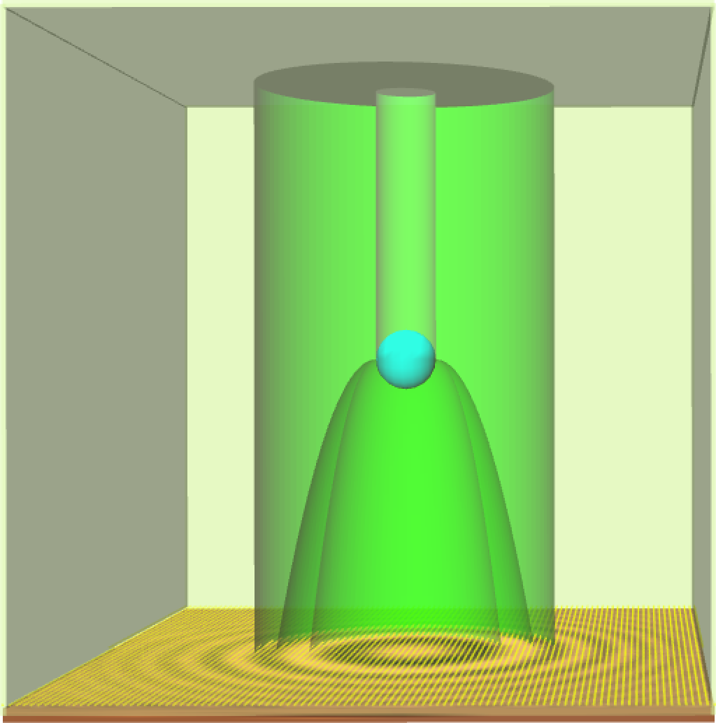
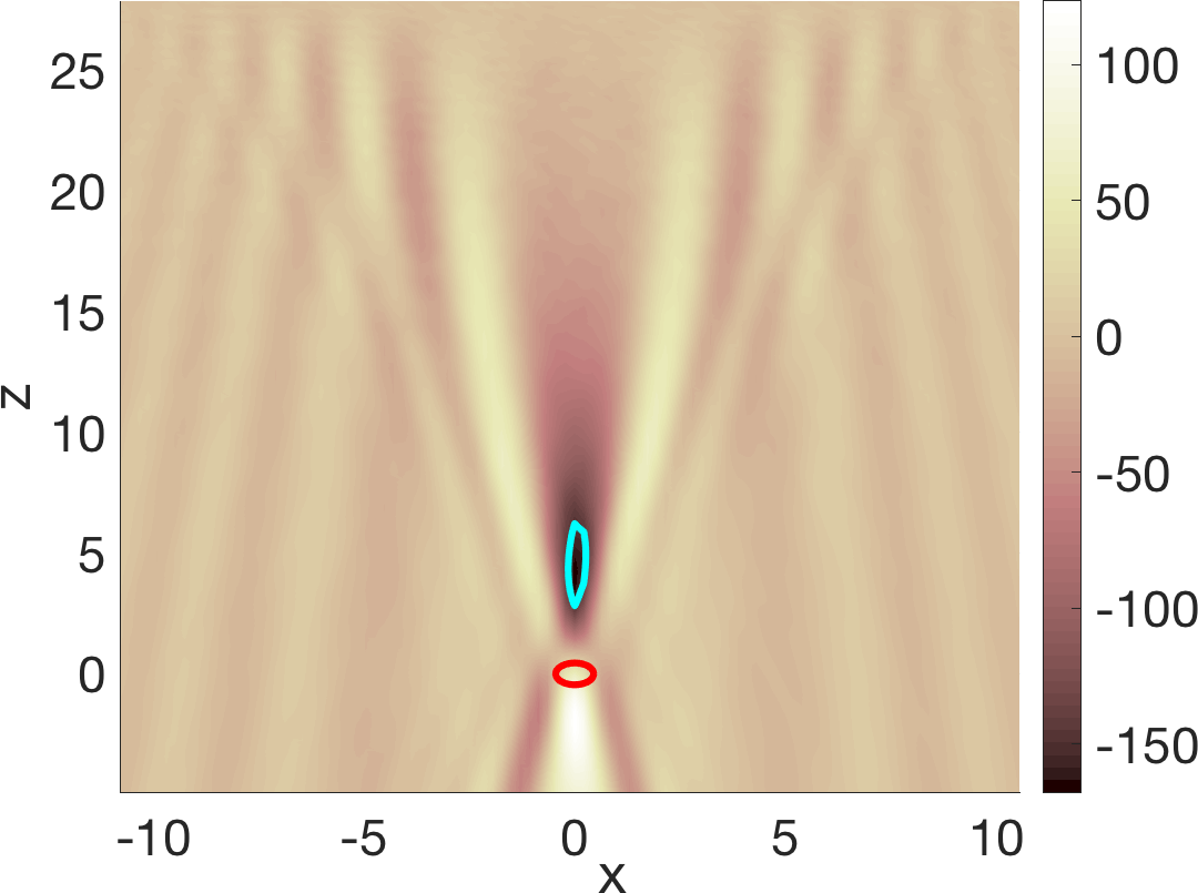
with $G_{{\kappa }_e}(\mathbf{x})=\frac{1}{4\pi |\mathbf{x}|}{e}^{ı{\kappa }_e|\mathbf{x}|}$ denoting the outgoing Green function of the Helmholtz equation [⁠31⁠ J.-C. Nédélec, Acoustic and electromagnetic equations. Appl. Math. Sci. 144, Springer, New York (2001) ]. Once ${\Omega }_{\mathrm{ap}}$ is constructed, we fit aparametrized contour ${\mathbf{q}}_{\mathrm{ap}}$ to its boundary. Starshaped parametrizations are typical choices. Figure ⁠2⁠ exemplifies the procedure. The method is robust to noise, in the sense that perturbations of the data with random 10 % or 20 % noise, for instance, produce similar results. Notice that the value of ${\kappa }_i$ enters through a factor that we may scale out in (⁠5⁠) and it is not really needed to localize the object. Similar results are obtained using the topological energy [⁠6⁠ A. Carpio, T. G. Dimiduk, M. L. Rapún and V. Selgas, Noninvasive imaging of three-dimensional micro and nanostructures by topological methods. SIAM J. Imaging Sci. 9, 1324–1354 (2016) ]

which does not involve ${\kappa }_i$ at all. No knowledge of ${\kappa }_i$ is needed to construct a first guess of the objects.

3.3 Regularized Gauss–Newton iterations

Fast methods to improve our knowledge of the objects starting from an initial guess are based on the following result. Let us consider two Hilbert spaces $X$, $Y$ and a Fréchet differentiable operator $\mathcal{F}:D(\mathcal{F})\subset X\to Y$. Assuming that the exact data $y\in Y$ are attainable (that is, there is $x\in X$ such that $\mathcal{F}(x)=y$), but only noisy data $y^{\delta }$ verifying $\Vert y^{\delta }-y{\Vert }_Y\le \delta$ are accessible, the iteratively regularized Gauss–Newton (IRGN) method [⁠1⁠ A. B. Bakushinskii, On a convergence problem of the iterative-regularized Gauss–Newton method. Zh. Vychisl. Mat. i Mat. Fiz. 32, 1503–1509 (1992) ] constructs a sequence $x_{k+1}^{\delta }$ as follows. We linearize the equation at $x_k^{\delta }$ at each step, approximate the solution of $\mathcal{F}(x_k^{\delta })+{\mathcal{F}}^{\prime }(x_k^{\delta })\xi =y^{\delta }$ through the minimization problem

and set $x_{k+1}^{\delta }=x_k^{\delta }+{\xi }_{k+1}$. The Tikhonov term ${\alpha }_k\Vert x_k^{\delta }+\xi -x_0{\Vert }_X^2$ has regularizing properties and promotes convergence for specific choices $x_0$ and ${\alpha }_k$ (see [⁠21⁠ T. Hohage, Logarithmic convergence rates of the iteratively regularized Gauss–Newton method for an inverse potential and an inverse scattering problem. Inverse Problems 13, 1279–1299 (1997) ]). The theory of linear Tikhonov regularization guarantees that

where ${\mathcal{F}}^{\prime }(x_k^{\delta }{)}^{\ast }$ denotes the adjoint of the Fréchet derivative ${\mathcal{F}}^{\prime }(x_k^{\delta })$. The noise level $\delta$ affects the stopping criterion, the so-called discrepancy principle.

In a holography set-up, the map $\mathcal{F}$ is the operator that to each parametrization of objects $\mathbf{q}$ assigns the synthetic hologram $\mathbf{I}(\mathbf{q})$ generated by solving the forward problem for those objects. Starshaped parametrizations are a standard choice for simple objects. They describe each object by a few parameters: its center and a radius function represented by a finite combination of spherical harmonics [⁠5⁠ A. Carpio, T. G. Dimiduk, F. Le Louër and M. L. Rapún, When topological derivatives met regularized Gauss–Newton iterations in holographic 3D imaging. J. Comput. Phys. 388, 224–251 (2019) , ⁠20⁠ H. Harbrecht and T. Hohage, Fast methods for three-dimensional inverse obstacle scattering problems. J. Integral Equations Appl. 19, 237–260 (2007) ]. Given a starshaped parametrization ${\mathbf{q}}_k$ and a recorded hologram ${\mathbf{I}}_{\mathrm{meas}}$ with a level of noise $\delta$, the IRGN method first solves the linearized equation

by addressing the nonlinear least squares problem

where $H^s({\mathbb{S}}^2)$, $s>0$, is an adequate Sobolev space [⁠5⁠ A. Carpio, T. G. Dimiduk, F. Le Louër and M. L. Rapún, When topological derivatives met regularized Gauss–Newton iterations in holographic 3D imaging. J. Comput. Phys. 388, 224–251 (2019) ], and then sets ${\mathbf{q}}_{k+1}={\mathbf{q}}_k+{\xi }_{k+1}$. The initial parametrization ${\mathbf{q}}_0={\mathbf{q}}_{\mathrm{ap}}$ represents the first guess of the objects constructed by topological methods. The updated objects ${\Omega }_k$ correspond to the parametrizations ${\mathbf{q}}_k$. The stopping criterion for the noise level $\delta$ is as follows. If the synthetic hologram calculated numerically for the current approximation of the objects $\mathbf{I}({\mathbf{q}}_k)$ satisfies

we stop the algorithm, $\tau >0$ being a parameter adjusted to guarantee a reasonable approximation while preventing early stops.

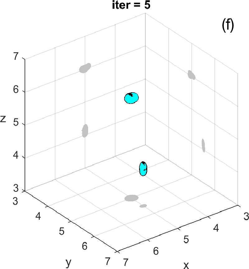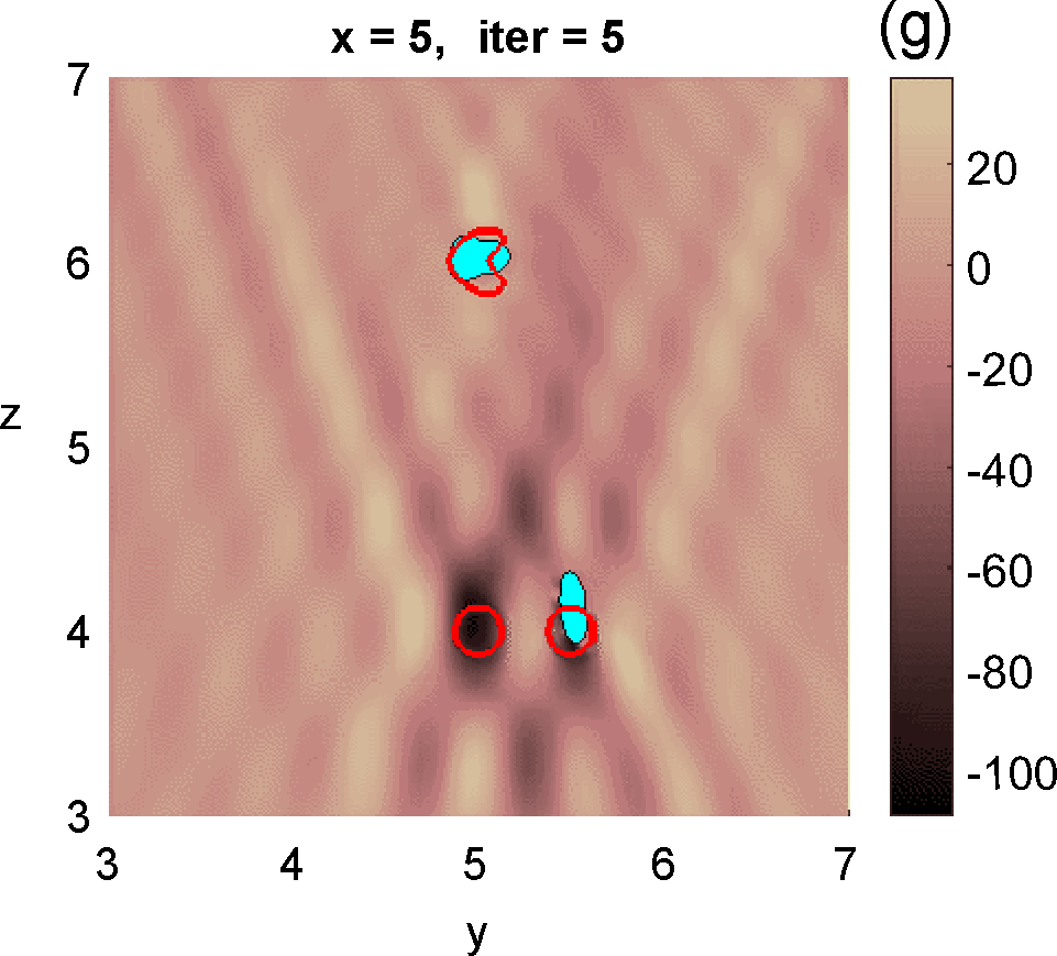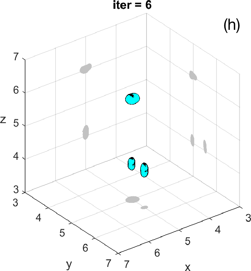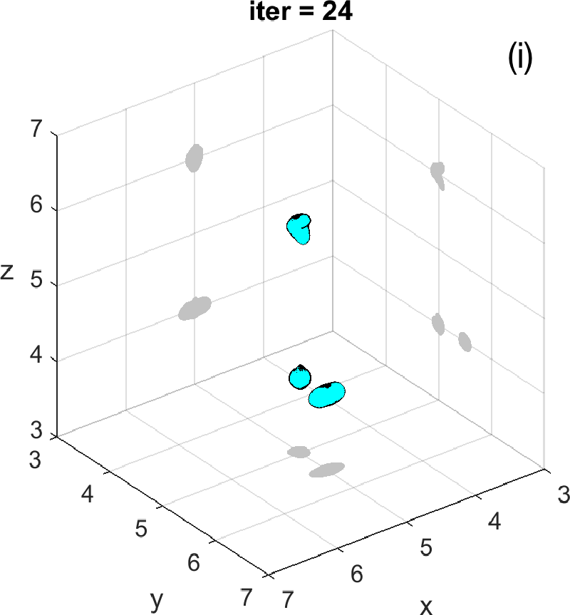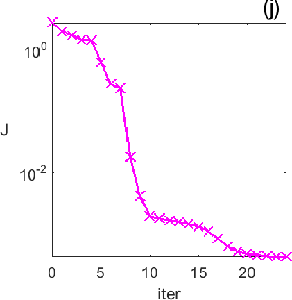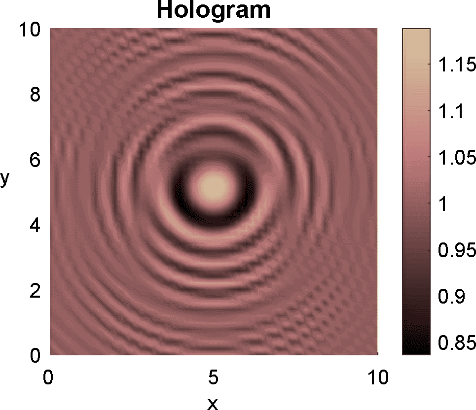
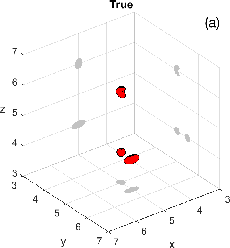
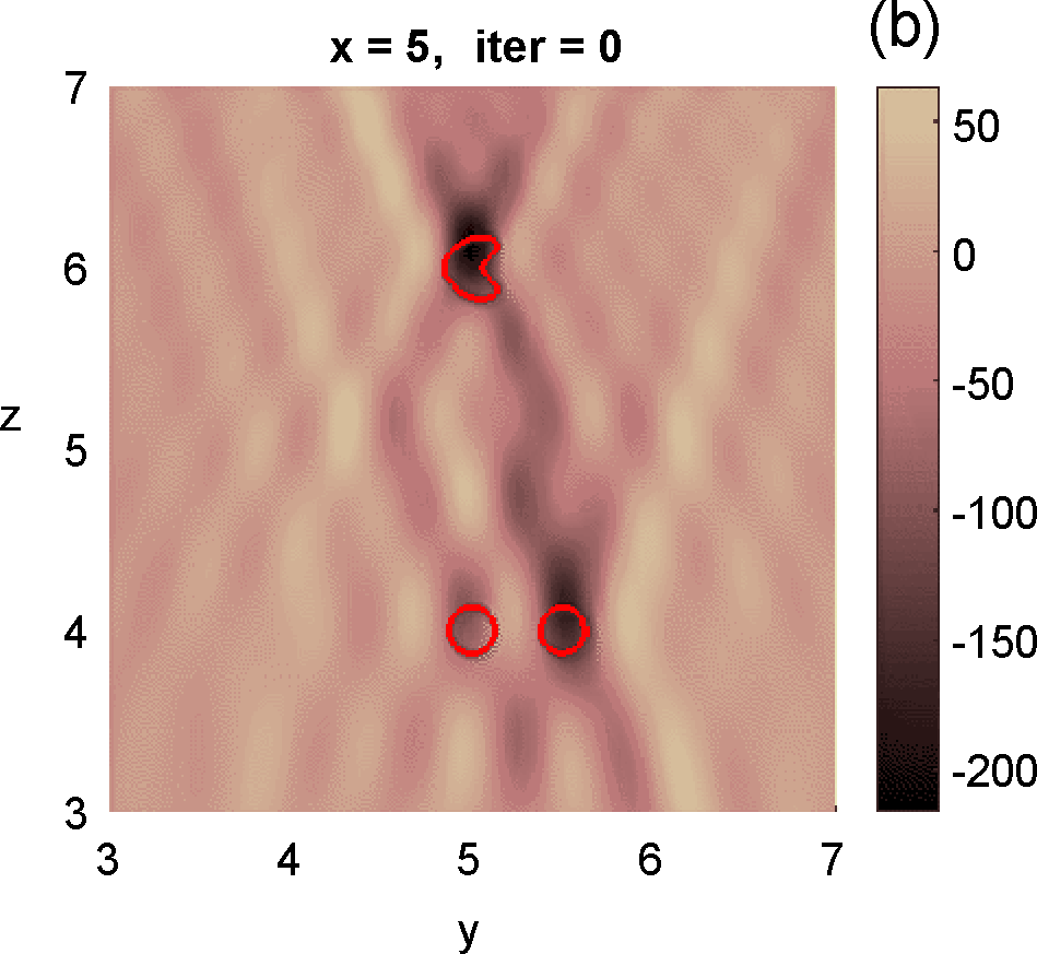
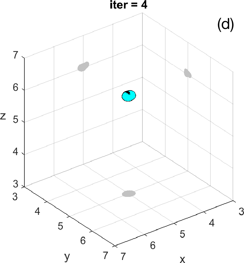
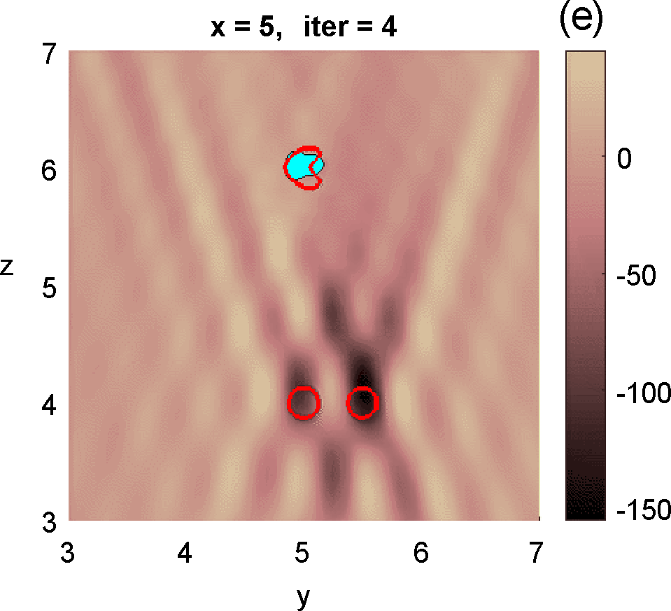
Figures ⁠3⁠ and ⁠4⁠ illustrate the process. Figure ⁠4⁠ depicts the hologram generated by the configuration with three objects shown in Figure ⁠3⁠ (a). We use the topological derivative (⁠5⁠) to spot a first dominant object at the top and locate an object there, see panel (b). Then we apply the IRGN method, see panels (c) and (d). At step 4 the cost functional, depicted in panel (j), stagnates without fulfilling the stopping criteria. This suggests that more objects should be created. This can be done by hybrid methods, as we explain next.

3.4 Topologically informed IRGN methods

Approaches that use initial object parametrization as reference have a drawback: the initial guess of the number of objects may be wrong. To overcome it, we have developed hybrid algorithms [⁠5⁠ A. Carpio, T. G. Dimiduk, F. Le Louër and M. L. Rapún, When topological derivatives met regularized Gauss–Newton iterations in holographic 3D imaging. J. Comput. Phys. 388, 224–251 (2019) ] combining topological derivatives and regularized Gauss–Newton iterations [⁠5⁠ A. Carpio, T. G. Dimiduk, F. Le Louër and M. L. Rapún, When topological derivatives met regularized Gauss–Newton iterations in holographic 3D imaging. J. Comput. Phys. 388, 224–251 (2019) ]. We fit an initial parametrization ${\mathbf{q}}_{\mathrm{ap}}$ to the first guess of the objects constructed by topological methods. Then, we apply the IRGN method and check that the cost (⁠2⁠) decreases. When the cost stagnates without fulfilling the stopping criteria, we reset ${\Omega }_{\mathrm{ap}}$ equal to the current guess of the objects ${\Omega }_k$ for the last parametrization obtained ${\mathbf{q}}_k$ and calculate the topological derivative of the cost for $\mathcal{R}={\mathbb{R}}^3\setminus \overline{{\Omega }_{\mathrm{ap}}}$. This is given by (⁠3⁠) if $\mathbf{x}\in \mathcal{R}={\mathbb{R}}^3\setminus \overline{\Omega }$ and its equivalent

if $\mathbf{x}\in \Omega$. Asymptotic calculations yield the formula [⁠9⁠ A. Carpio and M.-L. Rapún, Solving inhomogeneous inverse problems by topological derivative methods. Inverse Problems 24, Article ID 045014 (2008) , ⁠5⁠ A. Carpio, T. G. Dimiduk, F. Le Louër and M. L. Rapún, When topological derivatives met regularized Gauss–Newton iterations in holographic 3D imaging. J. Comput. Phys. 388, 224–251 (2019) ]

when ${\mu }_e={\mu }_i$, with forward and conjugate adjoint fields satisfying transmission Maxwell problems with object $\Omega ={\Omega }_{\mathrm{ap}}$:

where $\hat{\mathbf{n}}$ is the unit outer normal, $\hat{\mathbf{x}}=\mathbf{x}/|\mathbf{x}|$ and ${\delta }_{{\mathbf{x}}_j}$ are Dirac masses concentrated at the detectors ${\mathbf{x}}_j$, $j=1,...,N$.

We create a new approximation ${\Omega }_{\mathrm{new}}$ from ${\Omega }_{\mathrm{ap}}$ by removing the points in ${\Omega }_{\mathrm{ap}}$ at which the topological derivate surpasses a positive threshold $c_{\mathrm{new}}$ and adding the points outside ${\Omega }_{\mathrm{ap}}$ at which the topological derivate falls below a negative threshold $-C_{\mathrm{new}}$, see [⁠9⁠ A. Carpio and M.-L. Rapún, Solving inhomogeneous inverse problems by topological derivative methods. Inverse Problems 24, Article ID 045014 (2008) , ⁠6⁠ A. Carpio, T. G. Dimiduk, M. L. Rapún and V. Selgas, Noninvasive imaging of three-dimensional micro and nanostructures by topological methods. SIAM J. Imaging Sci. 9, 1324–1354 (2016) ]:

The constants $C_{\mathrm{new}}$, $c_{\mathrm{new}}$ are selected to ensure a decrease in the cost functional (⁠2⁠) keeping ${\kappa }_i$ fixed. Once ${\Omega }_{\mathrm{new}}$ is constructed, we fit a parametrization ${\mathbf{q}}_{\mathrm{new}}$ to its contour and restart the IRGN procedure for ${\mathbf{q}}_{\mathrm{ap}}={\mathbf{q}}_{\mathrm{new}}$. The procedure stops when the changes in the cost and the parametrizations fall below selected thresholds.

Let us revisit the example studied in Figures ⁠3⁠ and ⁠4⁠. At step 4 of the IRGN method the cost stagnates without fulfilling the stopping criteria. We calculate the topological derivative (⁠6⁠) of the cost for the current approximation of the objects, illustrated in Figure ⁠3⁠ (e). A new region where the topological derivative attains large negative values appears. We create a new object there and update the parametrization, see panel (f). Then we apply the IRGN method again. Since the cost functional still stagnates without fulfilling the stopping criteria, we recalculate the topological derivative (⁠6⁠) for the available object approximation. Panel (g) suggests the creation of a third object. We update the IRGN method using this new configuration, and evolve the resulting object configuration, represented in panel (h), until the stopping criterion is met at panel (i) after 24 steps. Panel (j) illustrates stagnation and decrease of the cost as new objects are added to the parametrization using topological information and the updated IRGN method evolves, in a logarithmic scale. These simulations assume ${\kappa }_i$ known and fixed. Once first guesses for ${\kappa }_i$ are available, we can implement this procedure considering constant values for ${\kappa }_i$ at each component of the parametrization. Obtaining first guesses for ${\kappa }_i$ that are reliable enough is a hard task [⁠7⁠ A. Carpio, T. G. Dimiduk, V. Selgas and P. Vidal, Optimization methods for in-line holography. SIAM J. Imaging Sci. 11, 923–956 (2018) ] and the optimization procedure can encounter difficulties. Bayesian approaches provide alternative procedures that can handle these difficulties while quantifying uncertainty associated to noise and missing information.

4 Bayesian inverse problem

Bayesian formulations consider all unknowns in the inverse problem as random variables. Given a recorded hologram ${\mathbf{I}}_{\mathrm{meas}}$, we seek a finite-dimensional vector of parameters $\nu$ characterizing the imaged objects. When we assume the presence of $L$ objects, $\nu$ is formed by $L$ blocks, one per object. Using Bayes’ formula [⁠22⁠ J. Kaipio and E. Somersalo, Statistical and computational inverse problems. Appl. Math. Sci. 160, Springer, New York (2005) , ⁠33⁠ A. Tarantola, Inverse problem theory and methods for model parameter estimation. Society for Industrial and Applied Mathematics (SIAM), Philadelphia (2005) ]

where $p_{\mathrm{pr}}(\nu )$ represents the prior probability of the variables, which incorporates our previous knowledge on them, while $p({\mathbf{I}}_{\mathrm{meas}}|\nu )$ is the conditional probability or likelihood of observing ${\mathbf{I}}_{\mathrm{meas}}$ given $\nu$. The solution of the Bayesian inverse problem is the posterior probability $p_{\mathrm{pt}}(\nu |{\mathbf{I}}_{\mathrm{meas}})$ of the parameters given the data. Sampling the posterior distribution, we obtain statistical information on the most likely values of the object parameters with quantified uncertainty.

4.1 Likelihood choice

Assuming additive Gaussian measurement noise, the measured hologram and the synthetic hologram obtained for the true object parameters are related by ${\mathbf{I}}_{\mathrm{meas}}=\mathbf{I}({\nu }_{\mathrm{true}})+\epsilon$, where the measurement noise $\epsilon$ is distributed as a multivariate Gaussian $\mathcal{N}(0,{\Gamma }_{\mathrm{n}})$ with zero mean and covariance matrix ${\Gamma }_{\mathrm{n}}$. A possible choice for the likelihood $p({\mathbf{I}}_{\mathrm{meas}}|\nu )$ is [⁠8⁠ A. Carpio, S. Iakunin and G. Stadler, Bayesian approach to inverse scattering with topological priors. Inverse Problems 36, Article ID 105001 (2020) ]

with $\Vert \mathbf{v}{\Vert }_{{\Gamma }_{\mathrm{n}}^{-1}}^2={\overline{\mathbf{v}}}^{\mathrm{t}}{\Gamma }_{\mathrm{n}}^{-1}\mathbf{v}$. Here, $\mathbf{I}(\nu )$ represents the synthetic hologram obtained solving the forward problem (⁠1⁠) for objects characterized by parameters $\nu$, see Section ⁠2⁠.

4.2 Topological priors

A typical choice for the prior distribution is a multivariate Gaussian

if $\nu$ is “admissible”, and $p_{\mathrm{pr}}(\nu )=0$ when $\nu$ is “not admissible”, that is, it does not satisfy known constraints on the parameter set, see [⁠8⁠ A. Carpio, S. Iakunin and G. Stadler, Bayesian approach to inverse scattering with topological priors. Inverse Problems 36, Article ID 105001 (2020) ] for details. Here, ${\Gamma }_{\mathrm{pr}}$ is the covariance matrix and $n$ is the total number of parameters characterizing the objects. The mean ${\nu }_0$ is typically a set of parameter values characterizing an initial guess of the objects. Sharp priors are obtained fitting parametrizations to first guesses of the objects obtained from the study of topological fields associated to deterministic shape costs, as explained in Section ⁠3.2⁠.

4.3 Markov chain Monte Carlo sampling

Combining (⁠7⁠), (⁠8⁠) and (⁠9⁠), the posterior probability becomes (neglecting normalization constants)

when $\nu$ is admissible, and $p_{\mathrm{pt}}(\nu )=0$ otherwise. Markov chain Monte Carlo (MCMC) methods provide tools to sample unnormalized posteriors. Classical MCMC methods, such as Hamiltonian Monte Carlo or Metropolis–Hastings [⁠30⁠ R. M. Neal, MCMC using Hamiltonian dynamics. In Handbook of Markov Chain Monte Carlo, edited by S. Brooks, A. Gelman, G. L. Jones and X. L. Meng, Chapman & Hall/CRC Handb. Mod. Stat. Methods, CRC Press, Boca Raton, 113–162 (2011) ] construct a chain of $n$-dimensional states ${\nu }^{(0)}\to {\nu }^{(1)}\to \cdots \to {\nu }^{(k)}\to \cdots$ which evolve to be distributed in accordance with the target distribution $p_{\mathrm{pt}}(\nu )$. After sampling an initial state ${\nu }^{(0)}$ from the prior distribution (⁠9⁠), the chain advances from one state ${\nu }^{(k)}$ to the next ${\nu }^{(k+1)}$ by means of a transition operator that varies with the method employed [⁠30⁠ R. M. Neal, MCMC using Hamiltonian dynamics. In Handbook of Markov Chain Monte Carlo, edited by S. Brooks, A. Gelman, G. L. Jones and X. L. Meng, Chapman & Hall/CRC Handb. Mod. Stat. Methods, CRC Press, Boca Raton, 113–162 (2011) ]. More recent ensemble MCMC samplers [⁠13⁠ M. M. Dunlop and G. Stadler, A gradient-free subspace-adjusting ensemble sampler for infinite-dimensional Bayesian inverse problems, preprint, arXiv:2202.11088v1 (2022) , ⁠18⁠ J. Goodman and J. Weare, Ensemble samplers with affine invariance. Commun. Appl. Math. Comput. Sci. 5, 65–80 (2010) ] draw $W$ initial states from the prior distribution (the “walkers” or “particles”) and transition to new states while mixing the previous ones to generate several chains. This approach allows for parallelization and can handle multimodal posteriors [⁠8⁠ A. Carpio, S. Iakunin and G. Stadler, Bayesian approach to inverse scattering with topological priors. Inverse Problems 36, Article ID 105001 (2020) ].

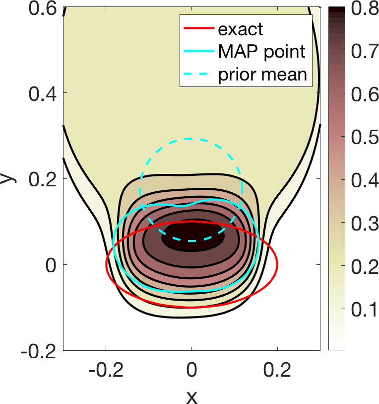
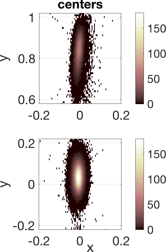
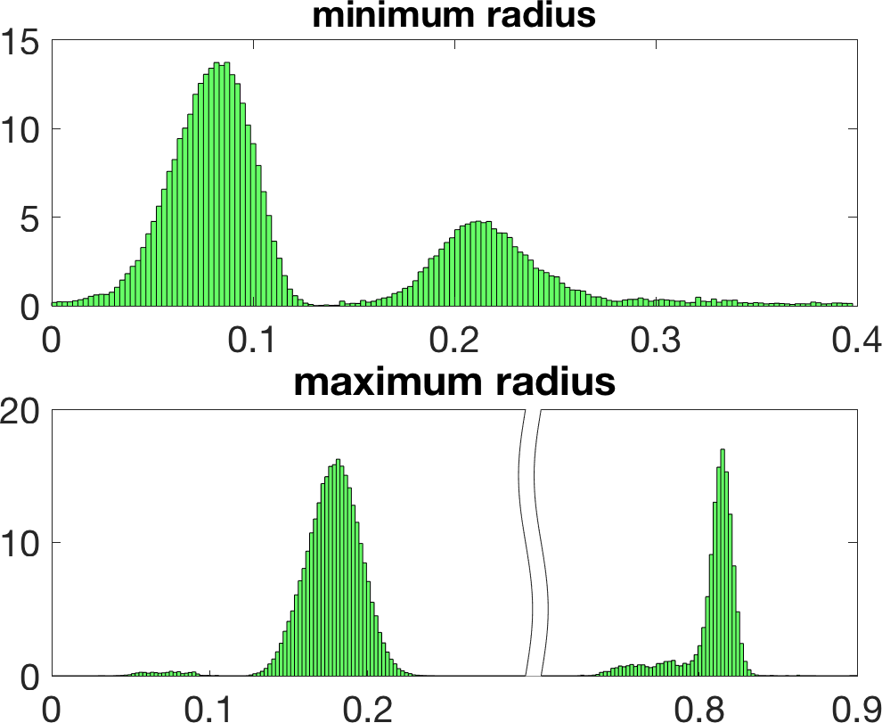
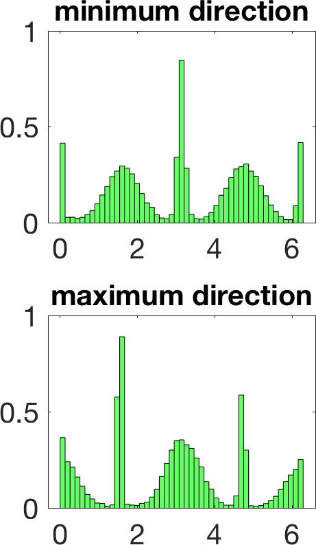
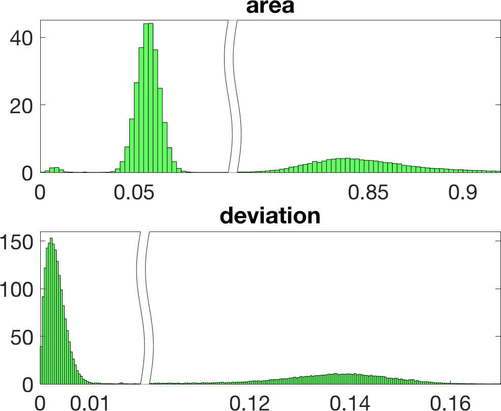
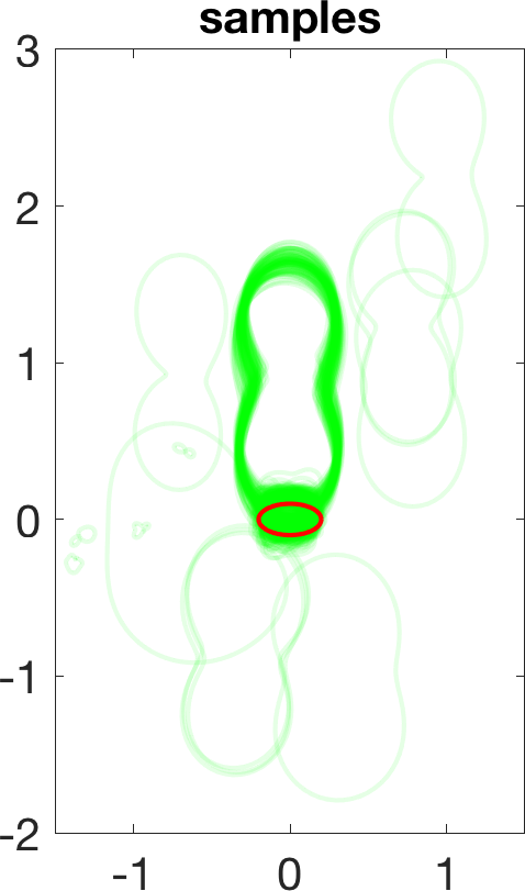
Figure ⁠5⁠ illustrates the results in a two-dimensional geometry, to reduce the computational cost in the tests. A few million samples were generated, which requires solving an identical number of forward problems. In two-dimensional set-ups we replace the stationary transmission problem for the Maxwell equations by a transmission problem posed for the Helmholtz equation [⁠8⁠ A. Carpio, S. Iakunin and G. Stadler, Bayesian approach to inverse scattering with topological priors. Inverse Problems 36, Article ID 105001 (2020) ]. Assuming ${\kappa }_i$ is piecewise constant, we resort to fast boundary elements to solve the Hemholtz transmission problems in two dimensions [⁠12⁠ V. Domínguez, S. Lu and F.-J. Sayas, A fully discrete Calderón calculus for two dimensional time harmonic waves. Int. J. Numer. Anal. Model. 11, 332–345 (2014) ]. Once a large enough collection of samples is generated [⁠17⁠ A. Gelman and D. B. Rubin, Inference from iterative simulation using multiple sequences. Statist. Sci. 7, 457–472 (1992) ], we extract statistical information describing the imaged object: the most likely shapes, sizes, locations, as well as uncertainty in the predictions. While starshaped two-dimensional objects can be reasonably characterized with 10–20 parameters, three-dimensional objects require 80–90. Full characterization of the posterior probability by MCMC sampling becomes more expensive as the number of parameters and the time required to solve forward problems increase.

4.4 Laplace approximation

The full characterization of the posterior probability is a challenging and costly probability problem for moderate- and high-dimensional parameters $\nu$. Low-cost approximations of the posterior distribution often rely on finding the maximum a posteriori (MAP) point, that is, the set of parameters that maximize the posterior probability. Upon taking logarithms, maximizing the posterior probability of the parameter set $\nu$ given the data ${\mathbf{I}}_{\mathrm{meas}}$ is equivalent to minimizing the regularized cost functional [⁠2⁠ C. M. Bishop, Pattern recognition and machine learning. Springer, New York (2006) ]

This is a nonlinear least-squares problem of the form previously considered in deterministic inversion, including regularization terms provided by the prior knowledge. We can solve it efficiently by using an adapted Levenberg–Marquardt–Fletcher iterative scheme [⁠15⁠ R. Fletcher, Modified Marquardt subroutine for non-linear least squares. Technical report 197213 (1971) ]. Starting from ${\nu }^0={\nu }_0$, we set ${\nu }^{k+1}={\nu }^k+{\xi }^{k+1}$, where ${\xi }^{k+1}$ is the solution of

Here, ${\mathbf{H}}^{\mathrm{GN}}$ is the Gauss–Newton approximation to the Hessian of the functional (⁠10⁠) and $\mathbf{g}$ is its gradient, while ${\lambda }_k$ is a scaling factor for ${\Gamma }_{\mathrm{pr}}^{-1}$ that balances the different orders of magnitude of the two terms defining the cost in the first iterations, and becomes equal to 1 at a certain point. At each step, the adjustable parameter ${\omega }_k>0$ increases until the cost $J({\nu }^k)$ decreases, and decreases otherwise, making the iteration closer to Gauss–Newton or gradient schemes as required.

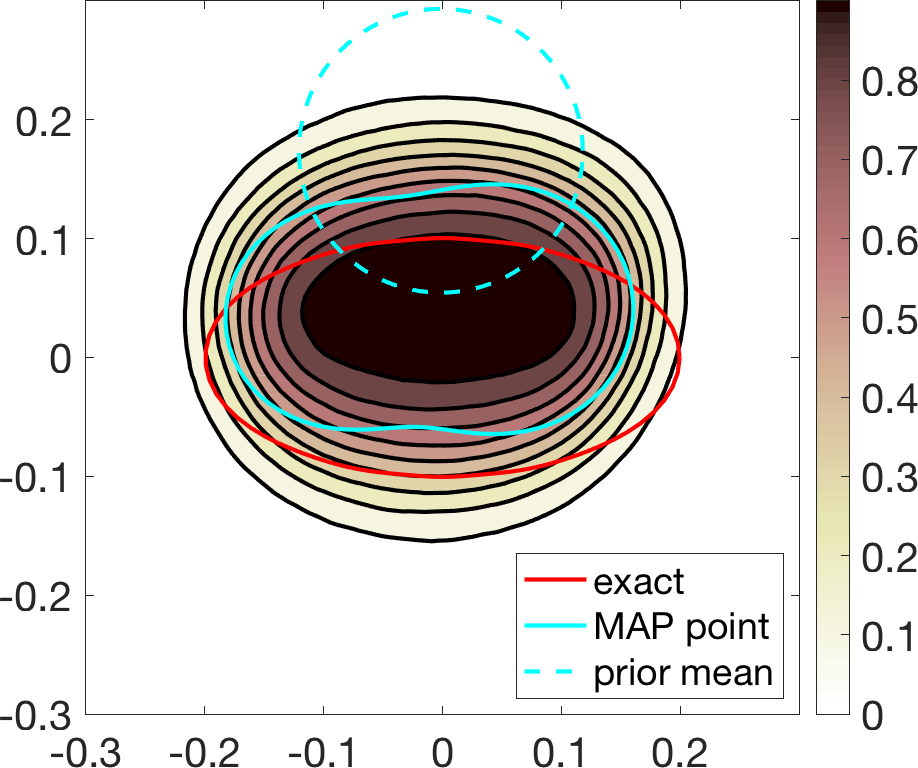
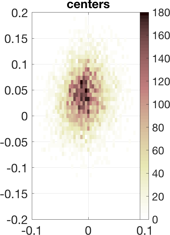
Linearization about the resulting MAP point ${\nu }_{\mathrm{MAP}}$ (the so-called Laplace approximation) provides an approximation of the posterior distribution by a Gaussian with mean ${\nu }_{\mathrm{MAP}}$ and posterior covariance ${\Gamma }_{\mathrm{po}}={\mathbf{H}}^{\mathrm{GN}}({\nu }_{\mathrm{MAP}}{)}^{-1}$. Sampling this Gaussian, we extract statistical information representing the dominant mode at a much lower computational cost, see Figure ⁠6⁠. Reaching ${\nu }_{\mathrm{MAP}}$ takes about 20 steps of scheme (⁠11⁠). The whole process, sampling included, is finished in a few minutes, instead of a few days.

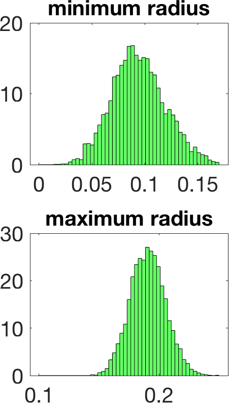
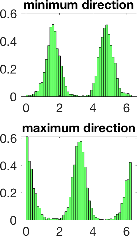
We have considered ${\kappa }_i$ fixed and known in these tests. In case it is constant and unknown, it becomes an additional parameter included in $\nu$. In the end, we obtain additional histograms reflecting uncertainty about the value with highest probability [⁠8⁠ A. Carpio, S. Iakunin and G. Stadler, Bayesian approach to inverse scattering with topological priors. Inverse Problems 36, Article ID 105001 (2020) ].

5 Perspectives

Digital holography poses challenging inverse problems which provide an opportunity to develop and test a variety of analytical and computational tools. First guesses of imaged objects are obtained by calculating the topological derivative of misfit functionals comparing the true hologram and the synthetic holograms that would be generated for different object configurations according to the selected forward model. Such guesses are robust to noise in the data. To reduce dimensionality, one can characterize the imaged objects by means of starshaped parametrizations. In a deterministic framework, we have shown that hybrid schemes combining iteratively regularized Gauss–Newton methods with topological derivative initializations and updates lead to good reconstructions of simple object configurations in a few steps, using stopping criteria that take into account the expected level of noise in the data. We are able to quantify uncertainty in such predictions by resorting to Bayesian formulations with topological priors. In two dimensions, Markov chain Monte Carlo methods provide a complete characterization of the posterior probability of the observed hologram being that is generated by a few starshaped objects. Three-dimensional tests are affordable for very simple shapes, such as a sphere or a cylinder [⁠11⁠ T. G. Dimiduk and V. N. Manoharan, Bayesian approach to analyzing holograms of colloidal particles. Optics Express 24, 24045–24060 (2016) ]. Handling high-dimensional parametrizations, in three dimensions or just irregular shapes, requires the introduction of strategies to reduce the computational cost. Laplace approximations based on optimizing to find the highest probability parameter set and then linearizing the posterior probability about it to obtain a multivariate Gaussian distribution are useful tools for uncertainty quantification when there is a single dominant mode. Developing fast sampling methods which are robust as dimension grows would be an important step forward to handle more general situations.

Holography set-ups are particularly challenging due to the fact that a single incident wave is used. We have focused here on light imaging, though acoustic waves can also be used to resolve at different scales. We expect similar techniques to be useful in inverse scattering problems involving other types of waves and different emitter/receiver configurations, such as microwave imaging or elastography, for instance.

Acknowledgements. Thanks to Krzysztof Burnecki for the kind invitation to write this article. The author is indebted to the Kavli Institute Seminars at Harvard for the interdisciplinary communication environment that initiated this work, M. P. Brenner for hospitality while visiting Harvard University, R. E. Caflisch for hospitality while visiting the Courant Institute at New York University, V. N. Manoharan for discussions of light holography, and D. G. Grier for an introduction to acoustic holography. The work summarized here has been done in collaboration with Thomas G. Dimiduk (Harvard University and Tesla), María Luisa Rapún (Universidad Politécnica de Madrid), Virginia Selgas (Universidad de Oviedo), Frédérique Le Louër (Université de Technologie de Compiègne), Georg Stadler (New York University), and Sergei Iakunin (Universidad Complutense de Madrid, now at the Basque Center for Applied Mathematics). This research was partially supported by the FEDER/MICINN–AEI grants PID2020-112796RB-C21, MTM2017-84446-C2-1-R, Fundación Caja Madrid Mobility grants, and MICINN “Salvador de Madariaga” Mobility grant PRX18/00112.

Ana Carpio graduated in numerical analysis from Universidad del País Vasco in Spain. She holds a PhD in mathematics from Laboratoire Jacques Louis Lions (Université Paris VI, now Paris Sorbonne), and has been a postdoctoral fellow at the Oxford Centre for Industrial and Applied Mathematics. She is a recipient of the SEMA (Spanish Society of Applied Mathematics) Prize to Young Researchers. Since 2006, she is a professor of applied mathematics at Universidad Complutense de Madrid and a member of the Gregorio Millán Barbany Institute for Modelling and Simulation in Fluid Dynamics, Nanoscience and Industrial Mathematics at Universidad Carlos III de Madrid. Currently, she serves as a Spanish representative in the ECMI (European Consortium for Mathematics in Industry) Council. Her main topics of research nowadays are inverse problems and data driven computational models in biomedicine. ana_carpio@mat.ucm.es

References

1. A. B. Bakushinskii, On a convergence problem of the iterative-regularized Gauss–Newton method. Zh. Vychisl. Mat. i Mat. Fiz. 32, 1503–1509 (1992)
2. C. M. Bishop, Pattern recognition and machine learning. Springer, New York (2006)
3. C. F. Borhen and D. R. Huffman, Absorption and scattering of light by small particles. Wiley Sciences, John Wiley & Sons, Berlin (1998)
4. T. Bui-Thanh, O. Ghattas, J. Martin and G. Stadler, A computational framework for infinite-dimensional Bayesian inverse problems Part I: The linearized case, with application to global seismic inversion. SIAM J. Sci. Comput. 35, A2494–A2523 (2013)
5. A. Carpio, T. G. Dimiduk, F. Le Louër and M. L. Rapún, When topological derivatives met regularized Gauss–Newton iterations in holographic 3D imaging. J. Comput. Phys. 388, 224–251 (2019)
6. A. Carpio, T. G. Dimiduk, M. L. Rapún and V. Selgas, Noninvasive imaging of three-dimensional micro and nanostructures by topological methods. SIAM J. Imaging Sci. 9, 1324–1354 (2016)
7. A. Carpio, T. G. Dimiduk, V. Selgas and P. Vidal, Optimization methods for in-line holography. SIAM J. Imaging Sci. 11, 923–956 (2018)
8. A. Carpio, S. Iakunin and G. Stadler, Bayesian approach to inverse scattering with topological priors. Inverse Problems 36, Article ID 105001 (2020)
9. A. Carpio and M.-L. Rapún, Solving inhomogeneous inverse problems by topological derivative methods. Inverse Problems 24, Article ID 045014 (2008)
10. D. Colton and R. Kress, Inverse acoustic and electromagnetic scattering theory. Appl. Math. Sci. 93, Springer, Berlin (1992)
11. T. G. Dimiduk and V. N. Manoharan, Bayesian approach to analyzing holograms of colloidal particles. Optics Express 24, 24045–24060 (2016)
12. V. Domínguez, S. Lu and F.-J. Sayas, A fully discrete Calderón calculus for two dimensional time harmonic waves. Int. J. Numer. Anal. Model. 11, 332–345 (2014)
13. M. M. Dunlop and G. Stadler, A gradient-free subspace-adjusting ensemble sampler for infinite-dimensional Bayesian inverse problems, preprint, arXiv:2202.11088v1 (2022)
14. G. R. Feijoo, A new method in inverse scattering based on the topological derivative. Inverse Problems 20, 1819–1840 (2004)
15. R. Fletcher, Modified Marquardt subroutine for non-linear least squares. Technical report 197213 (1971)
16. J. Fung, R. P. Perry, T. G. Dimiduk and V. N. Manoharan, Imaging multiple colloidal particles by fitting electromagnetic scattering solutions to digital holograms. J. Quant. Spectroscopy Radiative Transfer 113, 212–219 (2012)
17. A. Gelman and D. B. Rubin, Inference from iterative simulation using multiple sequences. Statist. Sci. 7, 457–472 (1992)
18. J. Goodman and J. Weare, Ensemble samplers with affine invariance. Commun. Appl. Math. Comput. Sci. 5, 65–80 (2010)
19. P. Grisvard, Elliptic problems in nonsmooth domains. Classics Appl. Math. 69, SIAM, Philadelphia (2011)
20. H. Harbrecht and T. Hohage, Fast methods for three-dimensional inverse obstacle scattering problems. J. Integral Equations Appl. 19, 237–260 (2007)
21. T. Hohage, Logarithmic convergence rates of the iteratively regularized Gauss–Newton method for an inverse potential and an inverse scattering problem. Inverse Problems 13, 1279–1299 (1997)
22. J. Kaipio and E. Somersalo, Statistical and computational inverse problems. Appl. Math. Sci. 160, Springer, New York (2005)
23. S. H. Lee, Y. Roichman, G. R. Yi, S. H. Kim, S. M. Yang, A. van Blaaderen, P. van Oostrum and D. G. Grier, Characterizing and tracking single colloidal particles with video holographic microscopy. Optics Express 15, 18275–18282 (2007)
24. F. Le Louër, A spectrally accurate method for the direct and inverse scattering problems by multiple 3D dielectric obstacles. ANZIAM J. 59, E1–E49 (2018)
25. A. Maier, S. Steidl, V. Christlein, J. Hornegger, Medical imaging systems: An introductory guide. Springer (2018)
26. P. Marquet, B. Rappaz, P. J. Magistretti, E. Cuche, Y. Emery, T. Colomb and C. Depeursinge, Digital holographic microscopy: a noninvasive contrast imaging technique allowing quantitative visualization of living cells with subwavelength axial accuracy. Optics Letters 30, 468–478 (2005)
27. M. Masmoudi, J. Pommier and B. Samet, The topological asymptotic expansion for the Maxwell equations and some applications. Inverse Problems 21, 547–564 (2005)
28. S. W. McCandless and C. R. Jackson, Principles of synthetic aperture radar. In SAR Marine Users Manual, NOAA (2004)
29. S. Meddahi, F.-J. Sayas and V. Selgás, Nonsymmetric coupling of BEM and mixed FEM on polyhedral interfaces. Math. Comp. 80, 43–68 (2011)
30. R. M. Neal, MCMC using Hamiltonian dynamics. In Handbook of Markov Chain Monte Carlo, edited by S. Brooks, A. Gelman, G. L. Jones and X. L. Meng, Chapman & Hall/CRC Handb. Mod. Stat. Methods, CRC Press, Boca Raton, 113–162 (2011)
31. J.-C. Nédélec, Acoustic and electromagnetic equations. Appl. Math. Sci. 144, Springer, New York (2001)
32. J. Sokołowski and A. Żochowski, On the topological derivative in shape optimization. SIAM J. Control Optim. 37, 1251–1272 (1999)
33. A. Tarantola, Inverse problem theory and methods for model parameter estimation. Society for Industrial and Applied Mathematics (SIAM), Philadelphia (2005)
34. J. Tromp, Seismic wavefield imaging of Earth’s interior across scales. Nature Reviews Earth & Environment 1, 40–53 (2020)
35. T. Vincent, Introduction to holography. CRC Press (2012)
36. A. Wang, T. G. Dimiduk, J. Fung, S. Razavi, I. Kretzschmar, K. Chaudhary and V. N. Manoharan, Using the discrete dipole approximation and holographic microscopy to measure rotational dynamics of non-spherical colloidal particles. J. Quant. Spectroscopy Radiative Transfer 146, 499–509 (2014)
37. A. Yevick, M. Hannel and D. G. Grier, Machine-learning approach to holographic particle characterization. Optics Express 22, 26884–26890 (2014)
38. M. A. Yurkin and A. G. Hoekstra, The discrete-dipole-approximation code ADDA: Capabilities and known limitations. J. Quant. Spectroscopy Radiative Transfer 112, 2234–2247 (2011)