Solved and unsolved problems

The present column is devoted to Geometry/Topology.

I Six new problems – solutions solicited

Solutions will appear in a subsequent issue.

252

Prove that the space of unordered couples of distinct points of a circle is the (open) Möbius band. More formally, consider

and the equivalence relation on this space $(x,y)\equiv (y,x)$; prove that the quotient topological space is the (open) Möbius band.

Costante Bellettini (Department of Mathematics, University College London, UK)

253

In the Euclidean plane, let ${\gamma }_1$ and ${\gamma }_2$ be two concentric circles of radius respectively $r_1$ and $r_2$, with $r_1<r_2$. Show that the locus $\gamma$ of points $P$ such that the polar line of $P$ with respect to ${\gamma }_2$ is tangent to ${\gamma }_1$ is a circle of radius $r_2^2/r_1$.

Acknowledgement

I want to thank the professors who guided me in the first part of my career for giving me the ideas for these problems.

Paola Bonacini (Mathematics and Computer Science Department, University of Catania, Italy)

254

Let $A\subseteq {\mathbb{R}}^3$ be a connected open subset of Euclidean space, and suppose that the following conditions hold:

1. Every smooth irrotational vector field on $A$ admits a potential (i.e., it is the gradient of a smooth function).

2. The closure $\overline{A}$ of $A$ is a smooth compact submanifold of ${\mathbb{R}}^3$ (of course, with non-empty boundary).

Show that $A$ is simply connected. Does this conclusion hold even if we drop condition (2) on $A$?

Roberto Frigerio (Dipartimento di Matematica, Università di Pisa, Italy)

255

A regulus is a surface in ${\mathbb{R}}^3$ that is formed as follows: We consider pairwise skew lines ${\ell }_1,{\ell }_2,{\ell }_3\subset {\mathbb{R}}^3$ and take the union of all lines that intersect each of ${\ell }_1$, ${\ell }_2$, and ${\ell }_3$. Prove that, for every regulus $U$, there exists an irreducible polynomial $f\in \mathbb{R}[x,y,z]$ of degree two that vanishes on $U$.

Adam Sheffer (Department of Mathematics, Baruch College, City University of New York, NY, USA)

256

(Enumerative Geometry). How many lines pass through $4$ generic lines in a $3$-dimensional complex projective space $\mathbb{C}{\mathbb{P}}^3$?

Mohammad F. Tehrani (Department of Mathematics, University of Iowa, USA)

257

I learned about the following problem from Shmuel Weinberger. It can be viewed as a topological analogue of Arrow’s Impossibility Theorem.

(a) A group of $n$ friends have decided to spend their summer cottaging together on an undeveloped island, which happens to be a perfect copy of the closed 2-disk $D^2$. Their first task is to decide where on this island to build their cabin. Being democratically-minded, the friends decide to vote on the question. Each friend chooses his or her favourite point on $D^2$. The friends want a function that will take as input their $n$ votes, and give as output a suitable point on $D^2$ to build. They believe, to be reasonable and fair, their “choice” function should have the following properties:

• (Continuity) It should be continuous as a function $(D^2{)}^n\to D^2$. This means, if one friend changes their vote by a small amount, the output will change only a small amount.

• (Symmetry) The $n$ friends should be indistinguishable from each other. If two friends swap votes, the final choice should be unaffected.

• (Unanimity) If all $n$ friends chose the same point $x$, then $x$ should be the final choice.

For which values of $n$ does such a choice function exist?

(b) The friends’ second task is to decide where along the shoreline of the island they will build their dock. The shoreline happens to be a perfect copy of the circle $S^1$. Again, they decide to take the problem to a vote. For which values of $n$ does a continuous, symmetric, and unanimous choice function $(S^1{)}^n\to S^1$ exist?

These are special cases of the following general problem in topological social choice theory: given a topological space $X$, for what values of $n$ does $X$ admit a social choice function that is continuous, symmetric, and unanimous? In other words, when is there a function $A:X^n\to X$ satisfying

• $A$ is continuous,

• $A(x_1,\dots ,x_n)$ is independent of the ordering of $x_1,\dots ,x_n$, and

• $A(x,x,x,\dots ,x)=x$ for all $x\in X$?

Jenny Wilson (Department of Mathematics, University of Michigan, USA)

II Open problem

Embeddings of contact domains

by Yakov Eliashberg (Department of Mathematics, Stanford University, USA)

One of the cornerstones of symplectic topology, Gromov’s non-squeezing theorem, see [⁠6⁠ M. Gromov, Pseudo holomorphic curves in symplectic manifolds. Invent. Math. 82, 307–347 (1985) ], asserts that for $n>1$ the ball of radius $R>1$ in the standard symplectic space $({\mathbb{R}}^{2n},\omega ={\sum }_1^{n}d{x}_j\wedge d{y}_j)$ does not admit a symplectic embedding into the domain

while there is no volume constraints to do that. Since that time, the theory of symplectic embedding has made a lot of progress (see F. Schlenk’s survey [⁠8⁠ F. Schlenk, Symplectic embedding problems, old and new.  Bull. Amer. Math. Soc. (N.S.) 55, 139–182 (2018) ] for recent results).

The (non-)embedding results in contact geometry, which is an odd-dimensional analogue of symplectic geometry, are rarer; below, we discuss a few open problems.

Recall that a contact structure $\xi$ on an $(2n+1)$-dimensional manifold $M$ is a completely non-integrable hyperplane field. If $\xi$ is defined by a Pfaffian equation $\alpha =0$ for a differential $1$-form $\alpha$ (and such a form can always be found locally, and if $\xi$ is co-orientable even globally) then the complete non-integrability can be expressed by the condition that $\alpha \wedge d{\alpha }^n$ is a non-vanishing $(2n+1)$-form on $M$.

In this set of problems, we will restrict our attention to domains in the contact manifold $X:-{\mathbb{R}}^{2n}\times S^1$, $S^1=\mathbb{R}/\mathbb{Z}$, endowed with the contact structure

Given a bounded domain $U\subset {\mathbb{R}}^{2n}$, we set

and refer to $\hat{U}$ as a quantized domain $U$. We say that a domain ${\hat{U}}_1$ admits a contact embedding into a domain ${\hat{U}}_2$ if there is a contact isotopy $f_t:{\hat{U}}_1\to X$, starting with the inclusion $f_0:{\hat{U}}_1\hookrightarrow X$ such that $f_1({\hat{U}}_1)\subset {\hat{U}}_2$. Note that any Hamiltonian isotopy which moves $U_1$ into $U_2$ lifts to a contact isotopy moving ${\hat{U}}_1$ into ${\hat{U}}_2$. Hence we will refer to the problem of contact embeddings between the domains ${\hat{U}}_1$ and ${\hat{U}}_2$ as a quantized version of the corresponding symplectic embedding problem of $U_1$ to $U_2$.

Denote by $B^{2n}(R)$ the $2n$-dimensional open ball of radius $R$ and by $P(r_1,\dots ,r_k)$ the polydisk $B^2(r_1)\times \cdots \times B^2(r_n)\subset {\mathbb{R}}^{2n}$, where $0<r_1\le r_2\le \cdots \le r_n$. It was shown in [⁠3⁠ Y. Eliashberg, S. S. Kim and L. Polterovich, Geometry of contact transformations and domains: orderability versus squeezing. Geom. Topol. 10, 1635–1747 (2006) ] that if $\pi r_1^2<k<\pi r_2^2$ for any integer $k\ge 1$, then ${\hat{B}}^{2n}(r_2)$ does not admit a contact embedding into ${\hat{B}}^{2n}(r_1)$. Another theorem from [⁠3⁠ Y. Eliashberg, S. S. Kim and L. Polterovich, Geometry of contact transformations and domains: orderability versus squeezing. Geom. Topol. 10, 1635–1747 (2006) ] states that if $\pi R^2<1$, then ${\hat{B}}^{2n}(R)$ admits a contact embedding into ${\hat{B}}^{2n}(r)$ for any $r>0$. The former result was improved in [⁠2⁠ S.-F. Chiu, Nonsqueezing property of contact balls. Duke Math. J. 166, 605–655 (2017) , ⁠5⁠ M. Fraser, Contact non-squeezing at large scale in ℝ2⁢n×S1. Internat. J. Math. 27, 1650107 (2016) ] to show that for any $r_1<r_2$ with $\pi r_2^2>1$ there is no contact embedding of ${\hat{B}}^{2n}(r_2)$ into ${\hat{B}}^{2n}(r_1)$. Recall that Gromov’s symplectic width${\mathrm{Width}}_{\mathrm{Gr}}(U)$ of a domain $U\subset {\mathbb{R}}^{2n}$ can be defined as the supremum of $\pi {\rho }^2$ such that $B^{2n}(\rho )$ can be symplectically embedded into the domain $U$. The above results can be slightly generalized to the following statement, see [⁠3⁠ Y. Eliashberg, S. S. Kim and L. Polterovich, Geometry of contact transformations and domains: orderability versus squeezing. Geom. Topol. 10, 1635–1747 (2006) ].

If, for two domains $U_1,U_2\subset {\mathbb{R}}^{2n}$, we have

then the quantized domain ${\hat{U}}_2$ does not admit a contact embedding into ${\hat{U}}_1$.

Very little is known about embeddings of contact domains beyond the above results. Let us formulate a couple of concrete problems concerning quantized versions of some relatively old embedding results in symplectic topology. As we already mentioned above, many new obstructions to symplectic embeddings were found in recent years. It is unknown whether any of them hold in the quantized versions.

258*

Here we say that ${\hat{B}}^{2n}(R)$ admits a contact packing by $k$ quantized balls ${\hat{B}}^{2n}(r)$ if the disjoint union

admits a contact embedding into ${\hat{B}}^{2n}(R)$. Note that the corresponding symplectic packing problem was intensively studied beginning with the seminal paper by Gromov [⁠6⁠ M. Gromov, Pseudo holomorphic curves in symplectic manifolds. Invent. Math. 82, 307–347 (1985) ], where he proved that the packing of the ball $B^{2n}(R)$ with 2 disjoint balls $B^{2n}(r)$ is possible if and only if $R^2>2r^2$. For $n=2$, the problem was significantly advanced by D. McDuff and L. Polterovich in [⁠7⁠ D. McDuff and L. Polterovich, Symplectic packings and algebraic geometry. Invent. Math. 115, 405–434 (1994) ], and then completely solved by P. Biran in [⁠1⁠ P. Biran, Symplectic packing in dimension 4. Geom. Funct. Anal. 7, 420–437 (1997) ]. In the contact case, Problem 258* is completely open.

259*

Note that a theorem of Floer–Hofer–Wysocki, see [⁠4⁠ A. Floer, H. Hofer and K. Wysocki, Applications of symplectic homology. I. Math. Z. 217, 577–606 (1994) ], states that when $2r^2>R^2$ the symplectic embeddings $j,\psi :P(r,r)\to \mathbb{P}(R,R)$ are not symplectically isotopic.

III Solutions

245

We consider a setting where there is a set of $m$ candidates

and a set of $n$ voters $[n]=\{1,\dots ,n\}$. Each voter ranks all candidates from the most preferred one to the least preferred one; we write $a{\succ }_{i}b$ if voter $i$ prefers candidate $a$ to candidate $b$. A collection of all voters’ rankings is called a preference profile. We say that a preference profile is single-peaked if there is a total order $⊲$ on the candidates (called the axis) such that for each voter $i$ the following holds: if $i$’s most preferred candidate is $c$ and $a⊲b⊲c$ or $c⊲b⊲a$, then $b{\succ }_{i}a$. That is, each ranking has a single “peak”, and then “declines” in either direction from that peak.

(i) In general, if we aggregate voters’ preferences over candidates, the resulting majority relation may have cycles: e.g., if $a{\succ }_{1}b{\succ }_{1}c$, $b{\succ }_{2}c{\succ }_{2}a$ and $c{\succ }_{3}a{\succ }_{3}b$, then a strict majority (2 out of 3) voters prefer $a$ to $b$, a strict majority prefer $b$ to $c$, yet a strict majority prefer $c$ to $a$. Argue that this cannot happen if the preference profile is single-peaked. That is, prove that if a profile is single-peaked, a strict majority of voters prefer $a$ to $b$, and a strict majority of voters prefer $b$ to $c$, then a strict majority of voters prefer $a$ to $c$.

(ii) Suppose that $n$ is odd and voters’ preferences are known to be single-peaked with respect to an axis $⊲$. Consider the following voting rule: we ask each voter $i$ to report their top candidate $t(i)$, find a median voter $i^{\ast }$, i.e.,

and output $t(i^{\ast })$. Argue that under this voting rule no voter can benefit from voting dishonestly, if a voter $i$ reports some candidate $a\ne t(i)$ instead of $t(i)$, this either does not change the outcome or results in an outcome that $i$ likes less than the outcome of the truthful voting.

(iii) We say that a preference profile is 1D-Euclidean if each candidate $c_j$ and each voter $i$ can be associated with a point in $\mathbb{R}$ so that the preferences are determined by distances, i.e., there is an embedding $x:C\cup [n]\to \mathbb{R}$ such that for all $a,b\in C$ and $i\in [n]$, we have $a{\succ }_{i}b$ if and only if $|x(i)-x(a)|<|x(i)-x(b)|$. Argue that a 1D-Euclidean profile is necessarily single-peaked. Show that the converse is not true, i.e., there exists a single-peaked profile that is not 1D-Euclidean.

(iv) Let $P$ be a single-peaked profile, and let $L$ be the set of candidates ranked last by at least one voter. Prove that $|L|\le 2$.

(v) Consider an axis $c_1⊲\cdots ⊲c_m$. Prove that there are exactly $2^{m-1}$ distinct votes that are single-peaked with respect to this axis. Explain how to sample from the uniform distribution over these votes.

These problems are based on references [⁠12⁠ H. Moulin, Axioms of Cooperative Decision Making. Cambridge University Press, Cambridge (1991) ] (parts (i) and (ii)), [⁠10⁠ C. H. Coombs. Psychological scaling without a unit of measurement. Psychological Review 57, 145 (1950) ] (part (iii)) and [⁠9⁠ V. Conitzer, Eliciting single-peaked preferences using comparison queries. J. Artificial Intelligence Res. 35, 161–191 (2009) , ⁠13⁠ T. Walsh, Generating single peaked votes. arXiv:1503.02766 (2015) ] (part (v)); part (iv) is folklore. See also the survey [⁠11⁠ E. Elkind, M. Lackner and D. Peters. Structured preferences. In Trends in Computational Social Choice, edited by U. Endriss, Chapter 10, AI Access, 187–207 (2017) ].

Edith Elkind (University of Oxford, UK)

Solution by the proposer

(i) We can restrict the voters’ preferences to the set $\{a,b,c\}$; the reader can check that a restriction of a single-peaked profile to a subset of candidates remains single-peaked. We consider three cases depending on how $a$, $b$ and $c$ are ordered by the axis $⊲$.

1. $a⊲b⊲c$ or $c⊲b⊲a$. Then all voters who prefer $a$ over $b$ have $a$ as their top choice and hence prefer $a$ to $c$.

2. $b⊲a⊲c$ or $c⊲a⊲b$. All voters who prefer $c$ over $a$ have $c$ as their top choice and hence prefer $a$ to $b$; therefore, these voters are in minority.

3. $a⊲c⊲b$ or $b⊲c⊲a$. This is impossible: all voters who prefer $b$ to $c$ have $b$ as their top choice, so we have a strict majority preferring $b$ over $a$, a contradiction.

(ii) Suppose the winner under truthful voting is $a$. Consider a voter $i$. If $t(i)=a$, then $i$ cannot improve the outcome by lying. So suppose $t(i)⊲a$ (the case $a⊲t(i)$ is symmetric). If $i$ reports $a$ or some candidate $b$ with $b⊲a$, this does not change what the top choice of the median voter is, and hence does not change the outcome. If $i$ reports a candidate $c$ with $t(i)⊲c$, then the median voter may shift to the right, i.e., further away from $i$’s true top choice; as $i$’s preferences are single-peaked, this does not improve the outcome from her perspective.

(iii) Ordering the candidates by their position, i.e., placing $a$ before $b$ on the axis $⊲$ if $x(a)<x(b)$ results in an axis witnessing that the input profile is single-peaked. To show that the converse is not true, consider the following four votes:

This profile is single-peaked on $a⊲b⊲c⊲d$. Now, suppose for contradiction that it is 1D-Euclidean, i.e., it admits an embedding $x$. Consider the positions of the four voters $x(1),x(2),x(3),x(4)$. Assume without loss of generality that $x(b)<x(c)$. Then we have

(as voters 1 and 3 prefer $b$ to $c$) and

(as voters 2 and 4 prefer $b$ to $c$). But now consider the point $\frac{1}{2}(x(a)+x(d))$. Voters 1 and 2 have to be on one side of this point and voters 3 and 4 have to be on the other side of this point, because of their preferences over $a$ vs. $d$. But this is clearly impossible!

(iv) Assume without loss of generality that $P$ is single-peaked with respect to the axis $c_1⊲\cdots ⊲c_m$. Clearly, $P$ may contain a vote that ranks $c_1$ last or a vote that ranks $c_m$ last. But it cannot contain a vote that ranks some $c_i$ with $1<i<m$ last: if the top candidate in that vote is a $c_j$ with $j<i$, then this voter prefers $c_i$ to $c_m$, and if the top candidate in that vote is a $c_k$ with $k>i$, then this voter prefers $c_i$ to $c_1$.

(v) Induction. For $m=2$, we have $2=2^{2-1}$ orders, i.e., $c_1\succ c_2$ and $c_2\succ c_1$. Now suppose the claim has been proved for all $m^{\prime }<m$. A vote that is single-peaked on $c_1⊲\cdots ⊲c_m$ may have $c_1$ in the last position, with candidates in top $m-1$ positions forming a single-peaked vote with respect to $c_2⊲\cdots ⊲c_m$ ($2^{m-2}$ options) or it may have $c_m$ in the last position, with candidates in top $m-1$ positions forming a single-peaked vote with respect to $c_1⊲\cdots ⊲c_{m-1}$ ($2^{m-2}$ options). For sampling, we can build the vote bottom-up. At the first step, we fill the last position with $c_1$ or $c_m$, with probability $\frac{1}{2}$ each. Once $k$ positions have been filled, $1\le k\le m-1$, the not-yet-ranked candidates form a contiguous segment $c_1⊲\cdots ⊲c_j$ of the axis. We then fill position $k+1$ from the bottom with $c_i$ or $c_j$, with equal probability. This sampling is uniform, because the probability of generating a specific ranking is exactly $2^{-m+1}$: we make $m-1$ choice, and with probability $\frac{1}{2}$ each choice is consistent with the target ranking.

246

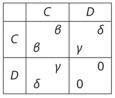
Consider a standard prisoners’ dilemma game described by the following strategic form, with $\delta >\beta >0>\gamma$:

Assume that any given agent either plays $C$ or $D$ and that agents reproduce at a rate determined by their payoff from the strategic form of the game plus a constant $f$. Suppose that members of an infinite population are assorted into finite groups of size $n$. Let $q$ denote the proportion of agents playing strategy $C$ (“altruists”) in the population as a whole and $q_i$ denote the proportion of agents playing $C$ in group $i$. We assume that currently $q\in (0,1)$.

The process of assortment is abstract, but we assume that it has finite expectation $E[q_i]=q$ and variance $\mathrm{Var}[q_i]={\sigma }^2$. Members within each group are then randomly paired off to play one iteration of the prisoners’ dilemma against another member of their group. All agents then return to the overall population.

1. Find a condition relating $q$, ${\sigma }^2$, $\beta$, $\gamma$, $\delta$ and $n$ under which the proportion of altruists in the overall population rises after a round of play.

2. Now interpret this game as one where each player can confer a benefit $b$ upon the other player by individually incurring a cost $c$, with $b>c>0$, so that $\beta =b-c$, $\delta =b$ and $\gamma =-c$. Prove that, as long as (i) there is some positive assortment in group formation and (ii) the ratio $\frac{c}{b}$ is low enough, then the proportion of altruists in the overall population will rise after a round of play.

Richard Povey (Hertford College and St Hilda’s College, University of Oxford, UK)

Solution by the proposer

(a) We can firstly see that the number of altruists (type $C$) and non-altruists (type $D$) in group $i$ after a round of play will be given by

Summing these two equalities yields

Given an infinite population and hence an infinite number of groups, the new proportion of altruists in the overall population will be

Substituting in $E[q_i^2]={\sigma }^2+E[q_i{]}^2$ and $E[q_i]=q$ gives us

Assuming $f$ is high enough to make the denominator positive, it then follows that

After some further rearrangement, we can derive the following:

Since the right-hand side of (⁠1⁠) must be strictly between $0$ and $1$, this has the intuitive interpretation that the inter-group variance ${\sigma }^2$ must be sufficiently high relative to the intra-group variance⁠¹⁠This is the variance of the Bernoulli variable $B(q)$ which takes a value of $1$ of a single individual drawn from the population is an altruist and $0$ otherwise, which is $q(1-q)$. so that, although altruists do less well relative to non-altruists within each group, the concentration of altruists together within particular groups is sufficiently strong to confer enough of an evolutionary advantage to offset this and to enable altruists to do better evolutionarily than non-altruists in the overall population.⁠²⁠This result was first proved in a general evolutionary context by George R. Price [⁠16⁠ G. R. Price, Selection and covariance, Nature 227, 520–521 (1970) , ⁠17⁠ G. R. Price, Extension of covariance selection mathematics, Ann. Human Genetics 35, 485–490 (1972) ].

(b) In the case where $\beta =b-c$, $\delta =b$ and $\gamma =-c$, condition (⁠1⁠) can be rearranged to give

With random assortment, $q_i$ would be equal to $\frac{X_i}{n}$ where $X_i$, the number of altruists in group $i$ would have a binomial distribution: $X_i\sim B(n,q)$. Therefore

With perfect positive correlation between group members, we would get

With some positive assortment generating positive covariance between group members, we may therefore without loss of generality suppose that

where $\epsilon \in (0,1)$. Plugging this into (⁠2⁠) and simplifying, we get $\frac{c}{b}<\epsilon$. So we can see that for any $\epsilon >0$ there always exists a value of $\frac{c}{b}$ low enough for altruists to expand as a proportion of the overall population.⁠³⁠The literature on this model has further established the results that multiple periods of isolation in finite groups acts to amplify inter-group variance, so that even with random assortment into groups altruism can evolve [⁠14⁠ B. Cooper and C. Wallace, Group selection and the evolution of altruism. Oxford Economic Papers 56, 307–330 (2004) ]. It has also been found that use of punishment strategies in dynamic interactions can act to weaken this group selection mechanism [⁠15⁠ R. Povey, Punishment and the potency of group selection, J. Evolutionary Economics 24 (2014) ]. For an accessible book-length treatment of the topic of group selection in the biological and social sciences, see [⁠18⁠ E. Sober and D. S. Wilson, Unto Others, Harvard University Press, Cambridge, Massachusetts (1999) ].

247

Consider a village consisting of n farmers who live along a circle of length $n$. The farmers live at positions $1,2,\dots ,n$. Each of them is friends with the person to the left and right of them, and each friendship has capacity $m$ where $m$ is a non-negative integer. At the end of the year, each farmer does either well (her wealth is $+1$ dollars) or not well (her wealth is $-1$ dollars) with equal probability. Farmers’ wealth realizations are independent of each other. Hence, for a large circle the share of farmers in each state is on average $1$.

The farmers share risk by transferring money to their direct neighbors. The goal of risk-sharing is to create as many farmers with OK wealth (0 dollars) as possible. Transfers have to be in integer dollars and cannot exceed the capacity of each link (which is $m$).

A few examples with a village of size $n=4$ serve to illustrate risk-sharing.

• Consider the case where farmers 1 to 4 have wealth

  $$(+1,-1,+1,-1).$$

  In that case, we can share risk completely with farmer $1$ sending a dollar to agent $2$ and farmer $3$ sending a dollar to farmer $4$. This works for any $m\ge 1$.

• Consider the case where farmers $1$ to $4$ have wealth

  $$(+1,+1,-1,-1).$$

  In that case, we can share risk completely with farmer $1$ sending a dollar to farmer $2$, farmer $2$ sending two dollars to farmer $3$ and farmer $3$ sending one dollar to farmer $4$. In this case, we need $m\ge 2$. If $m=1$, we can only share risk among half the people in the village.

Show that for any wealth realization an optimal risk-sharing arrangement can be found as the solution to a maximum flow problem.

Tanya Rosenblat (School of Information and Department of Economics, University of Michigan, USA)

Solution by the proposer

We augment the village graph by adding two auxiliary nodes. The source node$s$ is connected to all the farmers with positive wealth ($+1$) and each of these links has capacity $1$. The sink node$t$ is connected to all the farmers with negative wealth ($-1$) and each of these links also capacity $1$. We now look for the maximum flow from $s$ to $t$: this is equal to the number of luck/unlucky farmer pairs who can be matched under the best risk-sharing arrangement.

248

This exercise is a continuation of Problem 247 where we studied risk-sharing among farmers who live on a circle village and are friends with their direct neighbors to the left and right with friendships of a certain capacity. Assume that for any realization of wealth levels the best possible risk-sharing arrangement is implemented and denote the expected share of unmatched farmers with $U(n,m)$. Show that $U(n,m)\to \frac{1}{2m+1}$ as $n\to \infty$.

Tanya Rosenblat (School of Information and Department of Economics, University of Michigan, USA)

Solution by the proposer

The solution proceeds in two stages. In Problem 247, we already established that the problem can be understood as a maximum flow problem. We first formulate a particular algorithm that implements this flow. We then use this algorithm to express $U(n,m)$ in closed form.

Risk-sharing as a Maximum Flow Problem

We next describe a matching algorithm which is to run for $m$ rounds. The claim is that this algorithm implements the maximum flow in the augmented graph for any $m$. For the purpose of this algorithm, we call a black agent an agent with positive shock and a white agent an agent with a negative shock.

Step I: Index all agents from $1$ to $n$ clockwise ($1$ is the neighbor of $n$ on a circle). Set the counter $i$ to $1$.

Step II: If agents $i$ and $i+1$ are of different colors, label them “matched” and move the counter clockwise to $i+2$. If agent $i+1$ has the same color as agent $i$, then declare agent $i$ “unmatched” and move the counter clockwise to agent $i+1$. Repeat this step until the counter has reached the first agent again.

Step III: Define a new circle by ordering all the unmatched agents on a circle without disturbing the order of the agents. Essentially, this implies that all the matched agents are simply removed from the circle and any gaps are plugged by connected the closest unmatched agents with each other. Repeat steps I and II for this new circle. Repeat this algorithm $m$ times.

Proof. The Ford–Fulkerson algorithm computes the maximum flow by looking for open paths which can carry positive flow and then constructing a graph with augmented capacities in which the next path is found, etc. Once no more open path exists the max flow has been implemented. The above algorithm implements Ford–Fulkerson using a particular order of selecting open paths. Therefore, it implements the max flow.

Closed form solutions. We next prove the following lemma.

Proof. In each instance of step I of the algorithm, it produces an unmatched agent with probability $\alpha$ and a pair of matched agents with probability $1-\alpha$. The sum of unmatched and matched agents has to be $n$. Therefore the share of unmatched agents converges to

The final step in the proof of the result is to derive the probability ${\alpha }_m$ that an agent is followed by a same-color agent in round $m$. We know that in round $1$ shocks are i.i.d.; therefore ${\alpha }_1=\frac{1}{2}$. We start by proving a recursive formula for calculating ${\alpha }_m$.

Proof. Consider an agent $i$ on whom the counter rested at some point in the algorithm and who stays unmatched in the current round. This must be because he has a neighbor $i+1$ of the same color (without loss of generality assume both are black). With probability ${\alpha }_m$ agent $i+2$ is also black and therefore agent $i+1$ will survive into round $m+1$ as well and be of the same color as agent $i$ (black). With probability $1-{\alpha }_m$ agent $i+2$ is white. In this case agents $i+1$ and $i+2$ can be matched. Matching can continue for the subsequent pairs of agents $(i+3,i+4)$, $(i+5,i+6)$, etc.; it will only stop if for any of these pairs agents have the same color. This will happen with probability ${\alpha }_m$. To figure out it if this process will stop at a “white pair” or a “black pair” (let’s call it the “blocking pair”) it is crucial to know whether agent $i+2$, $i+4$, $i+6$, etc. (i.e., the agent just prior to the blocking pair) is white or black.

We know that agent $i+2$ is white. What is the probability that agent $i+4$ is the same color (provided $(i+3,i+4)$ is not a blocking pair)? This can only happen if the pair $(i+3,i+4)$ is a black agent followed by a white agent. If it is a white agent followed by a black agent then $i+4$ has a different color from $i+2$. So the probability of a color change is

Assume that the probability that the agent prior to the blocking pair is of the same color as $i+2$ is $q$. With probability ${\alpha }_m$ the pair $(i+3,i+4)$ is a blocking pair and with probability $1-{\alpha }_m$ the pair is not blocking. In that case agent $i+4$ has a different color from agent $i+2$ with probability ${\alpha }_m$. Because of the recursive nature of the problem, the probability that the agent prior to the blocking pair has the same color as $i+4$ is $q$. Therefore we know that

This allows us to calculate $q$ as

So we know that the agent prior to the blocking pair is white with probability $q$. The blocking pair is therefore a black blocking pair with probability $q(1-{\alpha }_m)+(1-q){\alpha }_m$. Therefore the total probability that the next unmatched agent after agent $i$ is of the same color (black in this case) is

We can check that ${\alpha }_m=1-\frac{1}{2m}$ satisfies both the initial condition and the recursive equation ⁠3⁠. This implies that

Finally, note that the share of unmatched agents (for $n\to \infty$) can be calculated by taking the product of the share of unmatched agents in each round:

249

In a combinatorial auction there are $m$ items for sale to $n$ buyers. Each buyer $i$ has some valuation function $v_i(\cdot )$ which takes as input a set $S$ of items and outputs that bidder’s value for that set. These functions will always be monotone ($v_i(S\cup T)\ge v_i(S)$ for all $S,T$), and satisfy $v_i(\varnothing )=0$.

Prove that a Walrasian equilibrium exists for $v_1,\dots ,v_n$ if and only if there exists an integral⁠⁴⁠That is, a point such that each $x_{i,S}\in \{0,1\}$. optimum to the following linear program:

Hint. Take the dual, and start from there.

Matt Weinberg (Computer Science, Princeton University, USA)

Solution by the proposer

First, we take the dual of the given LP. We use the dual variable $p_j$ for the constraints involving items, and the dual variable $u_i$ for the constraints involving bidders. Then the dual problem is

Walrasian equilibrium implies integral optimum

Now, assume that a Walrasian equilibrium exists, and let it be $p_1,\dots ,p_m$ and $B_1,\dots ,B_n$. Then consider the integral solution to the LP that sets $x_{i,B_i}=1$ for all $i$, and all other variables to $0$. This solution is clearly feasible for the LP, and has objective value equal to ${\sum }_i{v}_i(B_i)$.

Consider also the dual solution $u_i:-v_i(B_i)-{\sum }_{j\in B_i}{p}_j$, with $p_j$ as given in the Walrasian equilibrium. We claim this is a feasible solution to the dual. To see this, observe first that each $p_j\ge 0$. Also, because $B_i\in \arg {\max }_S\{v_i(S)-{\sum }_{j\in S}{p}_j\}$ by definition of Walrasian equilibrium, we have that

Therefore, all dual constraints are satisfied, and this is a feasible dual. Moreover, observe that the value of the dual objective is

The last equality follows because each item is in exactly one bundle $B_i$. So we have proved that if $(\vec{p},\vec{B})$ is a Walrasian equilibrium, then there is an integral feasible point for the LP with objective value ${\sum }_i{v}_i(B_i)$, and also a feasible dual solution with value ${\sum }_i{v}_i(B_i)$. By LP duality, both feasible solutions are in fact optimal. Therefore, there is an integral optimum for the LP.

Integral optimum implies Walrasian equilibrium

Now, assume that the LP has an integral optimum. Observe that for this integral solution, there must exist disjoint sets $B_1,\dots ,B_n$ such that for each $i$, $x_{i,B_i}=1$ and all other variables are $0$. The LP value for this solution is ${\sum }_i{v}_i(B_i)$. Moreover, observe that if any item $j\notin {\cup }_i{B}_i$, we can add $j$ to an arbitrary $B_i$ without decreasing ${\sum }_i{v}_i(B_i)$ (because each $v_i(\cdot )$ is monotone). Therefore, if there is an integral optimum to the LP, there exist disjoint $B_1,\dots ,B_n$ such that ${\cup }_i{B}_i=[m]$ and ${\sum }_i{v}_i(B_i)$ is the optimal solution to the LP.

By Strong LP Duality, there also exists a feasible dual solution $p_1,\dots ,p_m,u_1,\dots ,u_n$ such that ${\sum }_i{u}_i+{\sum }_j{p}_j={\sum }_i{v}_i(B_i)$. We will claim that $(\vec{p},\vec{B})$ form a Walrasian equilibrium.

For a proof by contradiction, assume that this is not the case. Then there must be some bidder $i$ such that $B_i\notin \arg {\max }_S\{v_i(S)-{\sum }_{j\in S}{p}_j\}$. In particular, this means that there exists some $B_i^{\prime }$ such that $v_i(B_i^{\prime })-{\sum }_{j\in B_i^{\prime }}>v_i(B_i)-{\sum }_{j\in B_i}$. Because $u_i$ is a feasible solution for the dual, we then conclude that

We claim that this contradicts the fact that ${\sum }_i{u}_i+{\sum }_j{p}_j={\sum }_i{v}_i(B_i)$, since