
1 Introduction
Vibration-based condition monitoring is commonly used for the maintenance of mechanical systems [35 R. B. Randall, Vibration-based condition monitoring: industrial, aerospace and automotive applications. John Wiley & Sons (2011) , 36 R. B. Randall and J. Antoni, Rolling element bearing diagnostics – a tutorial. Mech. Syst. Signal Process. 25, 485–520 (2011) ]. The main focus is usually set on gearboxes and bearings, as these elements appear in most transmission systems and their failure is the most frequent reason for a machine breakdown; for recent reviews, see [16 A. K. Jardine, D. Lin and D. Banjevic, A review on machinery diagnostics and prognostics implementing condition-based maintenance. Mech. Syst. Signal Process. 20, 1483–1510 (2006) , 42 Y. Wang, J. Xiang, R. Markert and M. Liang, Spectral kurtosis for fault detection, diagnosis and prognostics of rotating machines: A review with applications. Mech. Syst. Signal Process. 66, 679–698 (2016) ].
From the mathematical/statistical point of view, the task is defined as the detection of the periodic impulsive behaviour in the vibration signal. The most popular approach is the envelope analysis (and its various modifications) and detection of fault frequencies in the spectrum of the envelope for a given signal; see e.g. [5 P. Borghesani and J. Antoni, Cs2 analysis in presence of non-Gaussian background noise–effect on traditional estimators and resilience of log-envelope indicators. Mech. Syst. Signal Process. 90, 378–398 (2017) , 6 P. Borghesani and M. R. Shahriar, Cyclostationary analysis with logarithmic variance stabilisation. Mech. Syst. Signal Process. 70, 51–72 (2016) , 37 R. B. Randall, J. Antoni and S. Chobsaard, The relationship between spectral correlation and envelope analysis in the diagnostics of bearing faults and other cyclostationary machine signals. Mech. Syst. Signal Process. 15, 945–962 (2001) , 40 W. A. Smith, P. Borghesani, Q. Ni, K. Wang and Z. Peng, Optimal demodulation-band selection for envelope-based diagnostics: A comparative study of traditional and novel tools. Mech. Syst. Signal Process. 134, 106303 (2019) ]. The filtration of a raw signal is used to select its informative part and avoid other spectral content not related to the local damage.
The most popular approach is based on spectral kurtosis as an informative frequency band (IFB) selector (filter characteristic). The kurtosis value is calculated for sub-signal at some narrow frequency band. As kurtosis is sensitive to outliers [41 D. Wang, Some further thoughts about spectral kurtosis, spectral L2/L1 norm, spectral smoothness index and spectral gini index for characterizing repetitive transients. Mech. Syst. Signal Process. 108, 360–368 (2018) ], one can select impulsive content at a given narrow frequency band and filter out other components. Kurtosis is the most intuitive statistic commonly used for machine diagnostics [36 R. B. Randall and J. Antoni, Rolling element bearing diagnostics – a tutorial. Mech. Syst. Signal Process. 25, 485–520 (2011) ]. It has plenty of variations and extensions, e.g. the kurtogram [1 J. Antoni, Fast computation of the kurtogram for the detection of transient faults. Mech. Syst. Signal Process. 21, 108–124 (2007) ] which is a coloured map in which the depth of the colour values is proportional to the kurtosis value. Moreover, other statistics are also used in such context [33 J. Obuchowski, A. Wyłomańska and R. Zimroz, Selection of informative frequency band in local damage detection in rotating machinery. Mech. Syst. Signal Process. 48, 138–152 (2014) ].
In the literature, one can also find methods which are based on the cyclostationary approach. Recall that cyclostationary signals are considered when some of their characteristics are periodic in time. The most common characteristic used in this context is the autocovariance function, in which case we consider the cyclostationarity of the second order. The methods for the analysis of cyclostationary signals are dedicated to the cyclic behaviour identification. In the classical approach of cyclostationary-based techniques, the Gaussian distribution of the signal is usually assumed [2 J. Antoni, Cyclostationarity by examples. Mech. Syst. Signal Process. 23, 987–1036 (2009) , 6 P. Borghesani and M. R. Shahriar, Cyclostationary analysis with logarithmic variance stabilisation. Mech. Syst. Signal Process. 70, 51–72 (2016) , 7 F. Chaari, J. Leskow, A. Napolitane, R. Zimroz and A. Wylomanska, Cyclostationarity: theory and methods – IV. Springer (2020) , 11 V. Girondin, K. M. Pekpe, H. Morel and J.-P. Cassar, Bearings fault detection in helicopters using frequency readjustment and cyclostationary analysis. Mech. Syst. Signal Process. 38, 499–514 (2013) , 29 J. Lundén, S. A. Kassam and V. Koivunen, Robust nonparametric cyclic correlation-based spectrum sensing for cognitive radio. IEEE Trans. Signal Process. 58, 38–52 (2010) , 31 A. Napolitano, Cyclostationarity: New trends and applications. Signal Processing 120, 385–408 (2016) ].
One can also find other approaches for the informative frequency band selection based on artificial intelligence methods [26 R. Liu, B. Yang, E. Zio and X. Chen, Artificial intelligence for fault diagnosis of rotating machinery: A review. Mech. Syst. Signal Process. 108, 33–47 (2018) , 38 N. A. Salehzadeh and A. M. Ferri, Vibration-based techniques for damage detection and localization in engineering structures. World Scientific (2018) , 50 Y. Zhao, T. Li, X. Zhang and C. Zhang, Artificial intelligence-based fault detection and diagnosis methods for building energy systems: Advantages, challenges and the future. Renewable and Sustainable Energy Reviews 109, 85–101 (2019) ]. However, there is still a need for new approaches that would allow us to consistently handle restrictions linked to the amount of available data, specific type of noise, work specifications of the tested machine, etc.
Unfortunately, most of the standard statistical indicators used for local damage detection might be not appropriate in the presence of non-Gaussian noise. In the real environment, we observe signals with cyclic and impulsive behaviour. One of the examples is the crushing machine [47 A. Wyłomańska, R. Zimroz, J. Janczura and J. Obuchowski, Impulsive noise cancellation method for copper ore crusher vibration signals enhancement. IEEE Trans. Ind. Electron. 63, 5612–5621 (2016) ] used in mines. During the operation of such a machine (the crushing process), apart from the background noise (which is often assumed to be Gaussian white noise) in the vibration signal, large observations appear due to the nature of the machine’s work. Moreover, in the case of local damage, the additional cyclic impulses are hidden in the signal. In this case, the detection of local damage is very difficult. The non-Gaussian noise could be also linked to other technological processes of the working machine and may correspond to milling, sieving, cutting, compressing, etc. In the literature, algorithms for signals with non-Gaussian distribution have been proposed [10 G. Gelli, L. Izzo and L. Paura, Cyclostationarity-based signal detection and source location in non-Gaussian noise. IEEE Trans. Commun. 44, 368–376 (1996) , 19 J.-H. Jeon and Y.-H. Kim, Localization of moving periodic impulsive source in a noisy environment. Mech. Syst. Signal Process. 22, 753–759 (2008) , 21 V. Katkovnik, Robust m-periodogram. IEEE Trans. Signal Process. 46, 3104–3109 (1998) , 27 Y. Liu, T. Qiu and H. Sheng, Time-difference-of-arrival estimation algorithms for cyclostationary signals in impulsive noise. Signal Processing 92, 2238–2247 (2012) , 28 Y. Liu, Q. Wu, Y. Zhang, J. Gao and T. Qiu, Cyclostationarity-based DOA estimation algorithms for coherent signals in impulsive noise environments. EURASIP Journal on Wireless Communications and Networking 2019, 81 (2019) , 48 G. Yu, C. Li and J. Zhang, A new statistical modeling and detection method for rolling element bearing faults based on alpha–stable distribution. Mech. Syst. Signal Process. 41, 155–175 (2013) , 49 X. Zhao, Y. Qin, C. He, L. Jia and L. Kou, Rolling element bearing fault diagnosis under impulsive noise environment based on cyclic correntropy spectrum. Entropy 21, 50 (2019) ]. A new definition of the cyclostationary non-Gaussian signal was introduced in [25 P. Kruczek, R. Zimroz and A. Wyłomańska, How to detect the cyclostationarity in heavy-tailed distributed signals. Signal Processing 107514 (2020) ].
We demonstrate here some recently proposed algorithms for local damage detection that take into consideration the possible non-Gaussian behaviour of the signal and utilise the advanced statistics that are robust for large observations not related to failure. We present two approaches. The first is related to new techniques that can replace the classical measure of impulsiveness, i.e. kurtosis used as the selector for the IFB. In the second approach, the local damage is detected using the cyclostationary analysis dedicated to non-Gaussian distributed signals. All these techniques were recently published and used for simulated and real signals [12 J. Hebda-Sobkowicz, J. Nowicki, R. Zimroz and A. Wyłomańska, Alternative measures of dependence for cyclic behaviour identification in the signal with impulsive noise – application to the local damage detection. Electronics 10 (2021) , 13 J. Hebda-Sobkowicz, R. Zimroz, M. Pitera and A. Wylomanska, Informative frequency band selection in the presence of non-Gaussian noise – a novel approach based on the conditional variance statistic. Mech. Syst. Signal Process. 145 (2020) , 14 J. Hebda-Sobkowicz, R. Zimroz and A. Wyłomańska, Selection of the informative frequency band in a bearing fault diagnosis in the presence of non-Gaussian noise – comparison of recently developed methods. Applied Sciences 10 (2020) , 25 P. Kruczek, R. Zimroz and A. Wyłomańska, How to detect the cyclostationarity in heavy-tailed distributed signals. Signal Processing 107514 (2020) , 32 J. Nowicki, J. Hebda-Sobkowicz, R. Zimroz and A. Wyłomańska, Dependency measures for the diagnosis of local faults in application to the heavy-tailed vibration signal. Applied Acoustics 178, 107974 (2021) ]. Methods dedicated to non-Gaussian vibration signals were also developed during the OPMO project (EiT Raw Materials), which was carried out at the Wrocław University of Science and Technology (2019–2021), among others with a global mining industry leader KGHM. Those results were also the basis for two research projects currently implemented at the Faculty of Pure and Applied Mathematics at the Wrocław University of Science and Technology (the first in cooperation with the AMC Tech company and the second with the Tsinghua University, China).
2 Informative frequency band selectors for non-Gaussian signals
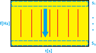
In the problem of IFB selection, the fist step is the decomposition of the raw signal into a set of narrow-band sub-signals using a time-frequency representation to obtain several dozen time series. To perform signal decomposition, one may use various techniques (wavelets, Wigner, EMD, etc.); see e.g. [9 Z. Feng, M. Liang and F. Chu, Recent advances in time–frequency analysis methods for machinery fault diagnosis: A review with application examples. Mech. Syst. Signal Process. 38, 165–205 (2013) ]. In this research, the Short-Time Fourier Transform (STFT) is used. The transform is defined as
where is the shift window, is the input signal, is its length, is the time point, and is a frequency; see [3 B. Boashash, Time-frequency signal analysis and processing: a comprehensive reference. Academic Press (2015) ] for more details. Interpretation of the STFT is intuitive: the squared envelope of the STFT (spectrogram) describes the energy flow in time for some narrow frequency band, i.e. sub-signal. The simplified representation of the spectrogram is presented in Figure 1 (a).
The next step is the application of some statistics (called selectors) to time series obtained from the spectrogram (Figure 1 (b)) to identify if a given sub-signal fulfils expectations regarding information about faults and select similar sub-signals from the whole frequency range. Distribution of selectors along frequencies, after normalisation, may constitute the filter characteristic (frequency response). One should expect that IFB for the healthy machine will contain stationary noise. In case of damage, the energy flow in some frequency bins will reveal a non-stationary character, and distribution of such sub-signals will be far from Gaussian; see [34 J. Obuchowski, R. Zimroz and A. Wylomanska, Identification of cyclic components in presence of non-Gaussian noise – application to crusher bearings damage detection. Journal of Vibroengineering 17 (2015) , 46 A. Wylomanska, R. Zimroz and J. Janczura, Identification and stochastic modelling of sources in copper ore crusher vibrations. In Journal of Physics: Conference Series, 628, IOP Publishing, 012125 (2015) , 47 A. Wyłomańska, R. Zimroz, J. Janczura and J. Obuchowski, Impulsive noise cancellation method for copper ore crusher vibration signals enhancement. IEEE Trans. Ind. Electron. 63, 5612–5621 (2016) ] for more details. In Figure 1, we present the general idea of preparing the signal to calculate the selectors for IFB using the time-frequency representation of the signal.
In the following subsections, we present three statistics that are considered in the literature as the IFB selectors.
2.1 Kurtosis
In probability theory and statistics, kurtosis is considered as the tail measure of the probability distribution [43 P. H. Westfall, Kurtosis as peakedness, 1905–2014. R.I.P. Amer. Statist. 68, 191–195 (2014) ]. For a given random variable with finite fourth moment, its kurtosis is defined as
where is the fourth central moment of , is its expectation of , and is the variance of . For a Gaussian random variable, the kurtosis is always equal to ; sometimes the term excess kurtosis is used in reference to . The empirical kurtosis is based on a scaled version of the fourth empirical moment of the data. Given a signal , the empirical kurtosis is a statistic defined as
where is the empirical sample variance and is the empirical mean; see [20 D. Joanes and C. Gill, Comparing measures of sample skewness and kurtosis. J. R. Stat. Soc. Ser. D Stat. 47, 183–189 (1998) ] for details. In our case, the statistic is calculated for the time series from time-frequency representation of the raw signal, see Figure 1 (b), and thus in this case it is called the spectral kurtosis [13 J. Hebda-Sobkowicz, R. Zimroz, M. Pitera and A. Wylomanska, Informative frequency band selection in the presence of non-Gaussian noise – a novel approach based on the conditional variance statistic. Mech. Syst. Signal Process. 145 (2020) ].
2.2 Alpha selector
Let us first recall the class of -stable distributions. It is considered as a natural extension (via the generalised limit theorem) of the classical Gaussian distribution; see [15 A. Janicki and A. Weron, Simulation and chaotic behavior of α-stable stochastic processes. Monographs and Textbooks in Pure and Applied Mathematics 178, Marcel Dekker, Inc., New York (1994) , 39 G. Samorodnitsky and M. S. Taqqu, Stable non-Gaussian random processes. Stochastic Modeling, Chapman & Hall, New York (1994) ]. It is very useful in data modelling with impulsive behaviour (also for damage detection), since in general it contains heavy-tailed (power-law) distributions. In the problem under consideration, we do not use the -stable distribution to describe the signal, but to analyse one of the parameters of this distribution (the stability index ) as the measure of impulsiveness, and consider its estimator as the selector for IFB.
The random variable has a stable distribution with stability index , scale parameter , skewness parameter , and shift parameter , if its characteristic function is given by
For , has a symmetric stable distribution, and for , the -stable distribution reduces to the Gaussian.
In the literature, one can find different estimation methods; see e.g. [4 S. Borak, W. Härdle and R. Weron, Stable distributions. In Statistical tools for finance and insurance, Springer, Berlin, 21–44 (2005) , 24 I. A. Koutrouvelis, Regression-type estimation of the parameters of stable laws. J. Amer. Statist. Assoc. 75, 918–928 (1980) ]. We use the classical McCulloch method [30 J. H. McCulloch, Simple consistent estimators of stable distribution parameters. Comm. Statist. Simulation Comput. 15, 1109–1136 (1986) ]. In further analysis, the statistic obtained using this approach applied to the sub-signals (Figure 1 (b)) is called the Alpha selector; see [13 J. Hebda-Sobkowicz, R. Zimroz, M. Pitera and A. Wylomanska, Informative frequency band selection in the presence of non-Gaussian noise – a novel approach based on the conditional variance statistic. Mech. Syst. Signal Process. 145 (2020) ].
2.3 Conditional variance-based selector
The selector called conditional variance-based (CVB) was introduced in [13 J. Hebda-Sobkowicz, R. Zimroz, M. Pitera and A. Wylomanska, Informative frequency band selection in the presence of non-Gaussian noise – a novel approach based on the conditional variance statistic. Mech. Syst. Signal Process. 145 (2020) ]. Below, we briefly describe this approach. Let us assume that is a Gaussian random variable with mean and standard deviation . Let denote the distribution function (cdf) of . For any level , we define the left, right, and middle quantile partitioning of by
where is the inverse of , i.e. denotes the -quantile of . Under the normality assumption and the partitioning ratio close to 20/60/20, i.e. for , we get that
where is the conditional variance of on set ; see [17 P. Jaworski and M. Pitera, The 20-60-20 rule. Discrete Contin. Dyn. Syst. Ser. B 21, 1149–1166 (2016) ] for details. Moreover, the ratio is the unique quantile (three set) partitioning satisfying property (1).
This property can be described as follows: if we split the large normal random sample into three sets, one corresponding to the worst (smallest) 20 % of outcomes, one corresponding to the middle 60 % of outcomes, and one corresponding to the best (largest) 20 % of outcomes, then the conditional variance on appropriate subsets is approximately the same.
As noted in [17 P. Jaworski and M. Pitera, The 20-60-20 rule. Discrete Contin. Dyn. Syst. Ser. B 21, 1149–1166 (2016) ], condition (1) creates a dispersion balance for the conditional populations. This might be linked to the statistical phenomenon commonly referred to as the 20/60/20 rule.
Since the ratio 20/60/20 is the unique ratio for which condition (1) is satisfied, it can be used to construct a goodness-of-fit test statistic. In other words, by comparing conditional variances with the conditional central variance, one can verify whether the sample comes from a Gaussian distribution. As the conditional tail variance might be seen as a measure of a tail heaviness, we can also use property (1) to benchmark any distribution tails with respect to normal tails without making any explicit assumptions about the distribution of .
The statistic used in [18 D. Jelito and M. Pitera, New fat-tail normality test based on conditional second moments with applications to finance. Statistical Papers 62, 2083–2108 (2020) ] for Gaussian distribution testing is defined as
where , is a normalisation constant, is the sample variance, and is set conditional sample variance. Assuming that the sample is independent and identically distributed, the asymptotic distribution of is standard normal. Moreover, if the sample under consideration comes from a (symmetric) heavy-tailed distribution, the values of the statistic should be positive due to high values of conditional tail variances on sets and . Consequently, could be considered as the measure of tail fatness, i.e. the bigger the value of , the fatter the tails. The value of for real signals is based on the empirical conditional variance. See [13 J. Hebda-Sobkowicz, R. Zimroz, M. Pitera and A. Wylomanska, Informative frequency band selection in the presence of non-Gaussian noise – a novel approach based on the conditional variance statistic. Mech. Syst. Signal Process. 145 (2020) ] for more details.
The statistic given in (2) can be extended, and a different number of partitioning sets could be considered. In [13 J. Hebda-Sobkowicz, R. Zimroz, M. Pitera and A. Wylomanska, Informative frequency band selection in the presence of non-Gaussian noise – a novel approach based on the conditional variance statistic. Mech. Syst. Signal Process. 145 (2020) ], it was proposed to partition into seven quantile conditioning subsets and use the (unique) ratio guaranteeing conditional variance equality. The statistic used as the CVB selector is defined as
where is the conditional sample variance on and the subsets come from the partitioning of the signal into seven appropriate subsets. In this approach, was used to measure the impact of the non-extreme (trimmed) tail variance on the central part of the distribution without bench-marking the model using Gaussian distribution. Similarly to what we saw above for kurtosis and the Alpha selector, applied to the time series (Figure 1 (b)) is used as the selector for IFB.
3 Comparative study of IFB selection – simulated signal analysis
In order to verify the efficiency of the presented selectors, we simulated four different types of signals: , , and . The first signal is the Gaussian white noise, which corresponds to the bearing vibration in a healthy condition; see Figure 6 (a). In such a case, we expect any of the informative frequency band selectors to respond significantly. The signal’s frequency is 25000 Hz and its length is 1 second. Signal corresponds to the locally damaged bearing vibration and is defined as
where is a unity-amplitude Gaussian radio-frequency (RF) pulse at the times indicated in array , with a centre frequency fc in hertz and a fractional bandwidth bw. ACI is the amplitude of the cyclic impulses (), is set to 2500 Hz, and the frequency modulation of cyclic impulses is equal to 30 Hz. The simulated signal is presented in Figure 6 (b).
The signal imitates the bearing operation of the loaded machine in a healthy condition; it is defined as
where is the amplitude of the non-cyclic impulses and is the location of the non-cyclic impulses, with the uniform distribution. The simulated signal is depicted in Figure 6 (c).
The last of the signals is a mixture of the previous ones, namely, it is defined as . It imitates the bearing vibrations in the case of a loaded machine operating in the unhealthy condition of bearing; see Figure 6 (d). In Figure 7, we present the spectrograms for the simulated signals presented in Figure 6. Panel (a) illustrates the spectrogram of the signal . The signal is the Gaussian white noise, so it is neither impulsive nor periodic. In panel (b), we demonstrate the spectrogram for signal . For this cyclic impulsive signal, we expect the techniques to point out the informative frequency band between 2 and 3 kHz (the centre frequency is set to 2500 Hz). In panel (c), we show the spectrogram for signal . For this non-cyclic impulsive signal, any IFB is expected. Finally, in panel (d), the spectrogram for signal is demonstrated. This is the most complicated case. The signal contains large non-cyclic and cyclic impulses. Thus, we expect to find information about the cyclic impulses with possibly suppressed information about non-cyclic ones.
In Figures 8–10, we present the considered selectors for the four simulated signals . As one can see, if the signal contains only the Gaussian noise (), all considered techniques, kurtosis, Alpha selectors and CVB, have relatively small amplitudes and do not indicate the informative frequency band, as expected. There is no frequency band which significantly stands out from the others. For the signal , all techniques work well, but the results for the CVB selector seem to be the most unequivocal. The value of the CVB selector in the range of the IFB is significantly higher than for other frequency bins. If the cyclic impulses have higher amplitudes, then their variance will increase and the value of the CVB will increase as well. For the non-cyclic impulsive signal , all techniques properly select the frequency band where the non-cyclic impulses appear. Note that none of the methods take into consideration the cyclic behaviour of the signal, only its impulsiveness. For the most complicated case, i.e. for the signal with a large non-cyclic to cyclic impulse amplitude ratio (), surprisingly only the CVB selector correctly identified the frequency band corresponding to the cyclic impulses, based on the distribution of their amplitudes. The kurtosis and Alpha selector indicate both cyclic and non-cyclic impulses frequency ranges. For more details and comparison with other selectors, see [14 J. Hebda-Sobkowicz, R. Zimroz and A. Wyłomańska, Selection of the informative frequency band in a bearing fault diagnosis in the presence of non-Gaussian noise – comparison of recently developed methods. Applied Sciences 10 (2020) ].
4 Real signal analysis
In this part, we present an application of the statistics we are considering to a real signal. The effectiveness of the different methods is verified on the data from the bearing of a crushing machine; see Figure 2.

All rights reserved.


However, due to the lack of local faults in the considered vibration data, we introduce an artificial component related to local damage. A similar approach was performed in [13 J. Hebda-Sobkowicz, R. Zimroz, M. Pitera and A. Wylomanska, Informative frequency band selection in the presence of non-Gaussian noise – a novel approach based on the conditional variance statistic. Mech. Syst. Signal Process. 145 (2020) , 44 J. Wodecki, P. Kruczek, A. Bartkowiak, R. Zimroz and A. Wyłomańska, Novel method of informative frequency band selection for vibration signal using nonnegative matrix factorization of spectrogram matrix. Mech. Syst. Signal Process. 130, 585–596 (2019) , 47 A. Wyłomańska, R. Zimroz, J. Janczura and J. Obuchowski, Impulsive noise cancellation method for copper ore crusher vibration signals enhancement. IEEE Trans. Ind. Electron. 63, 5612–5621 (2016) ]. The signal is presented in Figure 4. The length of the signal is 6 seconds and the sampling frequency is 25 kHz. The local fault was added with frequency modulation equal to 30 kHz and carrier frequency equal to 2.5 kHz (2–3 kHz). The spectrogram of the data is presented in Figure 11 (a). As we can see, the data reveals high-energy wide-band impulses around 0.25, 4.5 and 5.25 seconds, which correspond to falling rocks. The real vibration signal contains various components with a complex structure, and the component related to the damage is almost imperceptible above the noise. We apply the informative frequency band selectors to the real signal with its added fault. The results are presented in Figure 11 (b)–(d). The amplitude of the non-cyclic impulses is smaller than in the simulated data, but one can see that the results of the kurtosis fail. The Alpha selector properly indicates the IFB, but with much less selectivity than the CVB selector.
The signal filtered using the analysed selectors is presented in Figure 3. Filtering driven by the kurtosis selector (panel (a)) provides a single impulsive component that is a non-informative signal. In contrast, the Alpha selector (panel (b)) allows extraction of cyclic impulsive components with 2 random impulses. Finally, results of the CVB selector-based filtering (panel (c)) show a similar effect to the Alpha selector with slightly smaller random impulses. To summarise, Figure 3 shows that the filtration with the kurtosis selector fails, while the results of Alpha and CVB-based methods are acceptable and similar; however, we note that the shape of the CVB selector is better.
5 Cyclostationary analysis for non-Gaussian signals
In this part, we discuss new research related to the cyclostationary analysis for non-Gaussian signals. More precisely, we propose to apply dependency measures expressed by the known correlation coefficients to detect the cyclic behaviour on the time-frequency map. The idea is as follows. First, we represent the signal as the time-frequency map (Figure 1 (a)), then we consider the corresponding sub-signals as the separate time series (Figure 1 (b)), and finally, we apply the dependency measure (see examples below) to the time series extracted from the time-frequency representation of the signal. The general idea of this approach is illustrated in Figure 5.


5.1 Pearson correlation map
Let be a bi-dimensional sample of a random vector , where is the sample length. The Pearson correlation of is defined as follows [8 O. J. Dunn and V. A. Clark, Basic statistics: a primer for the biomedical sciences. John Wiley & Sons, Hoboken, NJ (2009) ]:
where is the covariance function, is the standard deviation of , and is the standard deviation of . The empirical equivalence of for , denoted , is defined as [8 O. J. Dunn and V. A. Clark, Basic statistics: a primer for the biomedical sciences. John Wiley & Sons, Hoboken, NJ (2009) ]
where , are sample means of data vectors and respectively. The Pearson correlation is usually a good dependency measure for finite-variance signals. However, this measure is sensitive to outliers. In our study, the Pearson correlation coefficient is applied to the sub-signals ; see Figure 1 (b).
5.2 Spearman correlation map
Let us again consider a bi-dimensional sample corresponding to a random vector Each pair and its empirical counterpart correspond to a pair and , where is the rank of the observation in the sample and is the rank of the observation in the sample . The Spearman rank correlation coefficient for the vector is defined as [23 M. G. Kendall, Rank correlation methods. Griffin (1948) ]
where is the covariance function, and are the standard deviations of the rank variables. The empirical version of the Spearman correlation coefficient is given by
where and are sample means in the relevant rank samples.
The Spearman correlation takes values in the interval and investigates a monotonic relationship, in contrast to the Pearson correlation, which analyses a linear relationship. Outliers do not disturb the Spearman correlation, whereas they do in the case of the Pearson correlation.
As we did for the Pearson correlation, in our study, we apply the Spearman correlation to the sub-signals ; see Figure 1 (b).
5.3 Kendall correlation map
The formula for the Kendall coefficient can be written as follows [22 M. G. Kendall, A new measure of rank correlation. Biometrika 30, 81–93 (1938) ]:
where
and if a pair is concordant with a pair i.e. if ; if a pair is discordant with a pair i.e. if
The Kendall correlation coefficient is based on the difference between the probability that two variables are in the same order (for the observed data vector) and the probability that their order is different. The Kendall coefficient indicates not only the strength but also the direction of the dependency. Like the Spearman correlation, it is resistant to outliers. In our study, the Kendall correlation is applied to the sub-signals from the time-frequency representation of the signal.
In the study [32 J. Nowicki, J. Hebda-Sobkowicz, R. Zimroz and A. Wyłomańska, Dependency measures for the diagnosis of local faults in application to the heavy-tailed vibration signal. Applied Acoustics 178, 107974 (2021) ], additional enhancements of the proposed dependency maps were proposed. We refer the readers to this position for more details.
6 Comparative study of dependency measure applications – analysis of simulated and real signals
In this section, we present results of IFB selection by using the above-mentioned dependency measures. The analyses are performed for the simulated signal , presented in Figure 6 (d). Recall that this is the signal that contains the non-Gaussian noise with cyclic impulses. In Figure 12, we present the enhanced dependency maps for the three correlation coefficients and for the signal by using the procedure presented in [32 J. Nowicki, J. Hebda-Sobkowicz, R. Zimroz and A. Wyłomańska, Dependency measures for the diagnosis of local faults in application to the heavy-tailed vibration signal. Applied Acoustics 178, 107974 (2021) ].
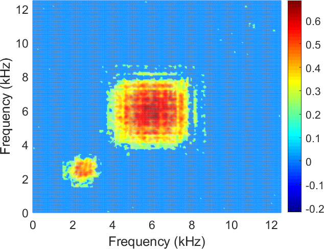
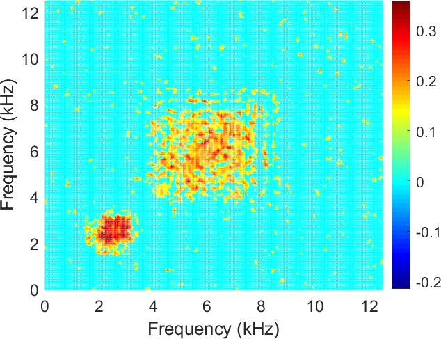
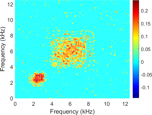
As one can see in Figure 12, in the case of the Pearson correlation map, the result differs from the other correlation maps. The correlation values at the location of the non-cyclic impulses are higher than for the cyclic impulses. In the other cases, one can see the opposite result. This result indicates that the application of more robust dependency measures may help to identify the cyclic impulsive behaviour in the case of impulsive noise.
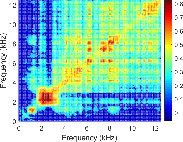
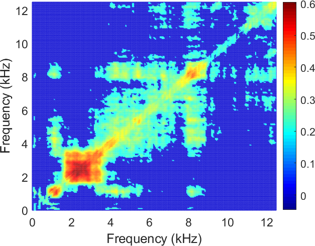
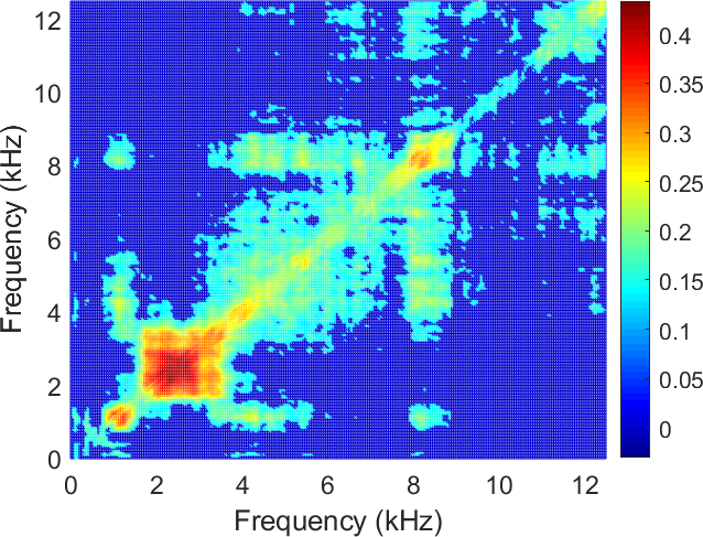
Finally, we apply the dependency measures to the real signal from the crushing machine presented in Section 4. The real signal is depicted in Figure 4. In Figure 13, we present the enhanced dependency maps based on the Pearson, Spearman and Kendall correlations discussed in the previous section. We can see that the clear picture can be obtained using the robust measures (i.e. Spearman and Kendall correlation maps), where the IFB is indicated properly. The Pearson correlation map reacts to the frequency band related to the non-cyclic impulses; thus it cannot be used as a proper measure for the cyclostationary analysis in the case of non-Gaussian noise. Related discussions are presented in [25 P. Kruczek, R. Zimroz and A. Wyłomańska, How to detect the cyclostationarity in heavy-tailed distributed signals. Signal Processing 107514 (2020) ].
Acknowledgements Let me thank Krzysztof Burnecki for the kind invitation to write this article. I would also like to thank Radosław Zimroz and the scientists in the Digital Mining Center (Faculty of Geoengineering, Mining and Geology at Wrocław University of Science and Technology, WUST) for our almost ten years of interdisciplinary research on new methods for real signal analysis. Thank you for showing me that mathematics can really be useful in practical applications, e.g. in the mining industry. Finally, I thank my PhD students and indeed all my students for providing new insights into our research, and positive energy.
The research was done within the Hugo Steinhaus Center at WUST whose goal is to organise, encourage and support research and education in numerical and stochastic techniques as applied in science and technology.
References
- J. Antoni, Fast computation of the kurtogram for the detection of transient faults. Mech. Syst. Signal Process. 21, 108–124 (2007)
- J. Antoni, Cyclostationarity by examples. Mech. Syst. Signal Process. 23, 987–1036 (2009)
- B. Boashash, Time-frequency signal analysis and processing: a comprehensive reference. Academic Press (2015)
- S. Borak, W. Härdle and R. Weron, Stable distributions. In Statistical tools for finance and insurance, Springer, Berlin, 21–44 (2005)
- P. Borghesani and J. Antoni, Cs2 analysis in presence of non-Gaussian background noise–effect on traditional estimators and resilience of log-envelope indicators. Mech. Syst. Signal Process. 90, 378–398 (2017)
- P. Borghesani and M. R. Shahriar, Cyclostationary analysis with logarithmic variance stabilisation. Mech. Syst. Signal Process. 70, 51–72 (2016)
- F. Chaari, J. Leskow, A. Napolitane, R. Zimroz and A. Wylomanska, Cyclostationarity: theory and methods – IV. Springer (2020)
- O. J. Dunn and V. A. Clark, Basic statistics: a primer for the biomedical sciences. John Wiley & Sons, Hoboken, NJ (2009)
- Z. Feng, M. Liang and F. Chu, Recent advances in time–frequency analysis methods for machinery fault diagnosis: A review with application examples. Mech. Syst. Signal Process. 38, 165–205 (2013)
- G. Gelli, L. Izzo and L. Paura, Cyclostationarity-based signal detection and source location in non-Gaussian noise. IEEE Trans. Commun. 44, 368–376 (1996)
- V. Girondin, K. M. Pekpe, H. Morel and J.-P. Cassar, Bearings fault detection in helicopters using frequency readjustment and cyclostationary analysis. Mech. Syst. Signal Process. 38, 499–514 (2013)
- J. Hebda-Sobkowicz, J. Nowicki, R. Zimroz and A. Wyłomańska, Alternative measures of dependence for cyclic behaviour identification in the signal with impulsive noise – application to the local damage detection. Electronics 10 (2021)
- J. Hebda-Sobkowicz, R. Zimroz, M. Pitera and A. Wylomanska, Informative frequency band selection in the presence of non-Gaussian noise – a novel approach based on the conditional variance statistic. Mech. Syst. Signal Process. 145 (2020)
- J. Hebda-Sobkowicz, R. Zimroz and A. Wyłomańska, Selection of the informative frequency band in a bearing fault diagnosis in the presence of non-Gaussian noise – comparison of recently developed methods. Applied Sciences 10 (2020)
- A. Janicki and A. Weron, Simulation and chaotic behavior of α-stable stochastic processes. Monographs and Textbooks in Pure and Applied Mathematics 178, Marcel Dekker, Inc., New York (1994)
- A. K. Jardine, D. Lin and D. Banjevic, A review on machinery diagnostics and prognostics implementing condition-based maintenance. Mech. Syst. Signal Process. 20, 1483–1510 (2006)
- P. Jaworski and M. Pitera, The 20-60-20 rule. Discrete Contin. Dyn. Syst. Ser. B 21, 1149–1166 (2016)
- D. Jelito and M. Pitera, New fat-tail normality test based on conditional second moments with applications to finance. Statistical Papers 62, 2083–2108 (2020)
- J.-H. Jeon and Y.-H. Kim, Localization of moving periodic impulsive source in a noisy environment. Mech. Syst. Signal Process. 22, 753–759 (2008)
- D. Joanes and C. Gill, Comparing measures of sample skewness and kurtosis. J. R. Stat. Soc. Ser. D Stat. 47, 183–189 (1998)
- V. Katkovnik, Robust m-periodogram. IEEE Trans. Signal Process. 46, 3104–3109 (1998)
- M. G. Kendall, A new measure of rank correlation. Biometrika 30, 81–93 (1938)
- M. G. Kendall, Rank correlation methods. Griffin (1948)
- I. A. Koutrouvelis, Regression-type estimation of the parameters of stable laws. J. Amer. Statist. Assoc. 75, 918–928 (1980)
- P. Kruczek, R. Zimroz and A. Wyłomańska, How to detect the cyclostationarity in heavy-tailed distributed signals. Signal Processing 107514 (2020)
- R. Liu, B. Yang, E. Zio and X. Chen, Artificial intelligence for fault diagnosis of rotating machinery: A review. Mech. Syst. Signal Process. 108, 33–47 (2018)
- Y. Liu, T. Qiu and H. Sheng, Time-difference-of-arrival estimation algorithms for cyclostationary signals in impulsive noise. Signal Processing 92, 2238–2247 (2012)
- Y. Liu, Q. Wu, Y. Zhang, J. Gao and T. Qiu, Cyclostationarity-based DOA estimation algorithms for coherent signals in impulsive noise environments. EURASIP Journal on Wireless Communications and Networking 2019, 81 (2019)
- J. Lundén, S. A. Kassam and V. Koivunen, Robust nonparametric cyclic correlation-based spectrum sensing for cognitive radio. IEEE Trans. Signal Process. 58, 38–52 (2010)
- J. H. McCulloch, Simple consistent estimators of stable distribution parameters. Comm. Statist. Simulation Comput. 15, 1109–1136 (1986)
- A. Napolitano, Cyclostationarity: New trends and applications. Signal Processing 120, 385–408 (2016)
- J. Nowicki, J. Hebda-Sobkowicz, R. Zimroz and A. Wyłomańska, Dependency measures for the diagnosis of local faults in application to the heavy-tailed vibration signal. Applied Acoustics 178, 107974 (2021)
- J. Obuchowski, A. Wyłomańska and R. Zimroz, Selection of informative frequency band in local damage detection in rotating machinery. Mech. Syst. Signal Process. 48, 138–152 (2014)
- J. Obuchowski, R. Zimroz and A. Wylomanska, Identification of cyclic components in presence of non-Gaussian noise – application to crusher bearings damage detection. Journal of Vibroengineering 17 (2015)
- R. B. Randall, Vibration-based condition monitoring: industrial, aerospace and automotive applications. John Wiley & Sons (2011)
- R. B. Randall and J. Antoni, Rolling element bearing diagnostics – a tutorial. Mech. Syst. Signal Process. 25, 485–520 (2011)
- R. B. Randall, J. Antoni and S. Chobsaard, The relationship between spectral correlation and envelope analysis in the diagnostics of bearing faults and other cyclostationary machine signals. Mech. Syst. Signal Process. 15, 945–962 (2001)
- N. A. Salehzadeh and A. M. Ferri, Vibration-based techniques for damage detection and localization in engineering structures. World Scientific (2018)
- G. Samorodnitsky and M. S. Taqqu, Stable non-Gaussian random processes. Stochastic Modeling, Chapman & Hall, New York (1994)
- W. A. Smith, P. Borghesani, Q. Ni, K. Wang and Z. Peng, Optimal demodulation-band selection for envelope-based diagnostics: A comparative study of traditional and novel tools. Mech. Syst. Signal Process. 134, 106303 (2019)
- D. Wang, Some further thoughts about spectral kurtosis, spectral L2/L1 norm, spectral smoothness index and spectral gini index for characterizing repetitive transients. Mech. Syst. Signal Process. 108, 360–368 (2018)
- Y. Wang, J. Xiang, R. Markert and M. Liang, Spectral kurtosis for fault detection, diagnosis and prognostics of rotating machines: A review with applications. Mech. Syst. Signal Process. 66, 679–698 (2016)
- P. H. Westfall, Kurtosis as peakedness, 1905–2014. R.I.P. Amer. Statist. 68, 191–195 (2014)
- J. Wodecki, P. Kruczek, A. Bartkowiak, R. Zimroz and A. Wyłomańska, Novel method of informative frequency band selection for vibration signal using nonnegative matrix factorization of spectrogram matrix. Mech. Syst. Signal Process. 130, 585–596 (2019)
- J. Wodecki, A. Michalak, A. Wyłomańska and R. Zimroz, Influence of non-Gaussian noise on the effectiveness of cyclostationary analysis – simulations and real data analysis. Measurement 171, 108814 (2021)
- A. Wylomanska, R. Zimroz and J. Janczura, Identification and stochastic modelling of sources in copper ore crusher vibrations. In Journal of Physics: Conference Series, 628, IOP Publishing, 012125 (2015)
- A. Wyłomańska, R. Zimroz, J. Janczura and J. Obuchowski, Impulsive noise cancellation method for copper ore crusher vibration signals enhancement. IEEE Trans. Ind. Electron. 63, 5612–5621 (2016)
- G. Yu, C. Li and J. Zhang, A new statistical modeling and detection method for rolling element bearing faults based on alpha–stable distribution. Mech. Syst. Signal Process. 41, 155–175 (2013)
- X. Zhao, Y. Qin, C. He, L. Jia and L. Kou, Rolling element bearing fault diagnosis under impulsive noise environment based on cyclic correntropy spectrum. Entropy 21, 50 (2019)
- Y. Zhao, T. Li, X. Zhang and C. Zhang, Artificial intelligence-based fault detection and diagnosis methods for building energy systems: Advantages, challenges and the future. Renewable and Sustainable Energy Reviews 109, 85–101 (2019)
Cite this article
Agnieszka Wyłomańska, Statistical tools for anomaly detection as a part of predictive maintenance in the mining industry. Eur. Math. Soc. Mag. 124 (2022), pp. 4–15
DOI 10.4171/MAG/66