
1 Geometry of surfaces
In this section we give a brief overview of some geometric facts regarding Riemann surfaces and K3 surfaces. Although both are called “surfaces”, Riemann surfaces are examples of algebraic curves, while K3 surfaces are genuine algebraic surfaces. This means that considering the complex points, Riemann surfaces are complex -dimensional while K3 surfaces are complex -dimensional. We will give some explicit examples and then describe geometric structures that live on these surfaces. In the Riemann case we are concerned with flat geometry (with singularities) while in the K3 case we consider Ricci-flat Kähler metrics. Moduli spaces of these geometric structures play an important role in the results of Section 2 below.
Riemann surfaces. One can describe a compact Riemann surface by giving the algebraic equations that cut it out in some ambient space. For example, consider
The locus of points satisfying this equation in is a real -dimensional surface of genus (with two points at infinity added to ). The -form from (1) is the unique (up to scale) holomorphic -form vanishing at the two points at infinity.
Flat geometry. There is an alternative way to describe the pair . Take the regular decagon in the plane and glue its opposite and parallel edges to form a surface of genus , with two marked points given by the vertices. If we identify the plane with , then the -form will be invariant under the translations used to glue opposite edges and will descend to a -form on the new surface. This construction gives back the same pair as described in (1), although this is by no means obvious. For more on the algebraic curve in (1), see [26 C. T. McMullen, Teichmüller curves in genus two: Torsion divisors and ratios of sines. Invent. Math.165, 651–672 (2006) , §5]. (A question for experts: what is the area of the decagon under this identification?)
This construction is quite general: starting from a pair consisting of a compact Riemann surface and a holomorphic -form, one can associate to it a polygon in the plane by cutting the surface and mapping it to the plane in such a way that in local charts the -form becomes . Equivalently, one can give charts to near a point by , and the transition maps between charts are translations in . Conversely, given a polygon in the plane (possibly disconnected), with side identifications given by translations, one can reconstruct a Riemann surface with a holomorphic -form using the converse to the above recipe.
Action of . A polygon is determined by its sides, which are vectors in . The group acts on polygons, keeping parallel sides parallel, so if we have a polygonal description of then we obtain a new pair . One can also express the action intrinsically on the surface, by letting a matrix act on the real and imaginary parts of , viewed as differential -forms on :
Note that the holomorphic structure on is usually different from the one on . Furthermore, even if explicit algebraic equations are given for , it is typically not possible to describe the equations cutting out . The sides of the polygons describing the surfaces are computed by taking integrals of on paths in , and the passage from algebraic equations to integrals and back is by no means explicit.
Moduli spaces of Riemann surfaces. Because algebraic equations have finitely many coefficients, one can consider full parameter spaces, or moduli spaces, of algebraic manifolds defined by the same type of equations. For Riemann surfaces we will be interested in the space of pairs where is a compact Riemann surface and is a holomorphic -form with describing the multiplicities of the zeros of . The process described above of obtaining a new pair using a real matrix gives an action of on . This action, however, is not via polynomial or even holomorphic automorphisms. In Section 2 we will see, however, that there are some relations between the -action and the algebraic equations defining Riemann surfaces.
For more on the -action on , see the surveys of Zorich [36 A. Zorich, Flat surfaces. In Frontiers in number theory, physics, and geometry. I, Springer, Berlin, 437–583 (2006) ] for an introduction as well as numerous motivations and applications, as well as the more recent surveys of Forni–Matheus [20 G. Forni and C. Matheus, Introduction to Teichmüller theory and its applications to dynamics of interval exchange transformations, flows on surfaces and billiards. J. Mod. Dyn.8, 271–436 (2014) ] and Wright [33 A. Wright, From rational billiards to dynamics on moduli spaces. Bull. Amer. Math. Soc. (N.S.)53, 41–56 (2016) ].
K3 surfaces. We now switch gears and consider algebraic surfaces, such as those given by the equation
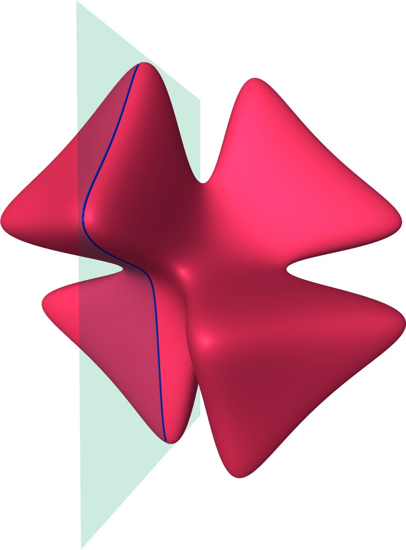
The -form is nowhere-vanishing on and is computed via a residue construction (take the residue of along ). It is interesting to consider both the complex and the real solutions of this equation, denoted and respectively. See Figure 1 for an example of real solutions. Algebraic curves (i.e., Riemann surfaces), such as those described in (1), have only finite automorphism groups as soon as the genus is at least two, but algebraic surfaces such as the one in (2) have dynamically interesting automorphisms such as
as well as their analogues in which the roles of the coordinates are permuted. The formula for the automorphism is obtained by “freezing” the and variables, viewing (2) as a quadratic equation for , and exchanging the two solutions of the quadratic. In particular applying twice gives back the identity transformation: .
Kähler geometry. The complex solutions of algebraic equations such as the ones above yield projective algebraic manifolds. These admit Kähler metrics, special kinds of Riemannian metrics adapted to the complex structure. For Kähler metrics, the Riemannian volume of an algebraic submanifold is determined by its homology class alone.
Specializing further, if the algebraic manifold admits an algebraic volume form, such as from (3), then Yau’s solution of the Calabi conjecture [34 S. T. Yau, On the Ricci curvature of a compact Kähler manifold and the complex Monge–Ampère equation. I. Comm. Pure Appl. Math.31, 339–411 (1978) ] gives canonical Kähler metrics whose Ricci curvature vanishes. To construct such metrics, one needs to solve a nonlinear PDE of Monge–Ampère type and there is no “hands-on” description of such metrics as in Figure 2.


Moduli spaces of K3 surfaces. Moving to algebraic manifolds of higher dimensions, additional data needs to be specified in order to have well-behaved moduli spaces. For us, the most relevant will be the space of Ricci-flat metrics on the manifold underlying a complex K3 surface. The abbreviation is for Kähler–Einstein, since Ricci-flat metrics satisfy the Einstein equation with . These moduli spaces play an essential role in the study of K3 surfaces and have the remarkable feature that they are (essentially) homogeneous spaces for appropriate Lie groups. For an introduction to the geometry of K3 surfaces, see the collection of notes [2 A. Beauville, Géométrie des surfaces K3: modules et périodes. Astérisque, Société Mathématique de France, Paris (1985) ] and the more recent monograph of Huybrechts [22 D. Huybrechts, Lectures on K3 surfaces. Cambridge Studies in Advanced Mathematics 158, Cambridge University Press, Cambridge (2016) ].
2 Dynamics on moduli spaces
This section describes results on the dynamics of group actions in the moduli space of Riemann and K3 surfaces equipped with appropriate flat, or Ricci-flat, metrics.
Dynamics on moduli spaces of flat surfaces. The action of the group on the moduli space of Riemann surfaces with a holomorphic -form satisfies rigidity properties akin to those for unipotent flows in homogeneous dynamics developed by Ratner [30 M. Ratner, On Raghunathan’s measure conjecture. Ann. of Math. (2)134, 545–607 (1991) , 31 M. Ratner, Raghunathan’s topological conjecture and distributions of unipotent flows. Duke Math. J.63, 235–280 (1991) ], Margulis [24 G. A. Margulis, Formes quadratriques indéfinies et flots unipotents sur les espaces homogènes. C. R. Acad. Sci. Paris Sér. I Math.304, 249–253 (1987) ] and many others. The following results were established by Eskin, Mirzakhani, and Mohammadi:
For any pair , the orbit closure is a submanifold of , described in local coordinates by linear relations among the sides of the polygons used to parametrize surfaces. Furthermore,1The switch from to is done to exclude the scaling action. any -invariant ergodic probability measure must be Lebesgue supported on such a manifold.
Going back to the algebraic description of Riemann surfaces, we saw that except in special symmetric situations, it is not possible in general to relate the algebraic equations to the polygonal description of the surface. In the case of -orbit closures, it is possible to give an alternative, purely algebraic description of their geometry. Specifically, recall that the Jacobian associated to a genus Riemann surface is the complex torus defined as , where denotes the complex -dimensional space of holomorphic -forms on , denotes the dual, and the first homology group embeds in the dual by integration along cycles. Alternatively, the Jacobian is the moduli space of holomorphic degree line bundles on and this description provides a link between the algebraic and analytic structures on a Riemann surface. Although the automorphism group of a genus Riemann surface is finite, the endomorphism group of its Jacobian can be much larger (real or complex multiplication give examples of such symmetries).
Orbit closures as in Theorem 1 parametrize Riemann surfaces whose Jacobians have additional endomorphisms a specific kind (such as real multiplication). Furthermore, specific combinations of the zeros of the distinguished -form yield torsion points on the Jacobian.
These conditions characterize as a locus inside .
Additional finiteness results for orbit closures are established in [6 A. Eskin, S. Filip and A. Wright, The algebraic hull of the Kontsevich–Zorich cocycle. Ann. of Math. (2)188, 281–313 (2018) ], jointly with Eskin and Wright.
The relation between the -action and real multiplication on Jacobians was discovered by McMullen [25 C. T. McMullen, Billiards and Teichmüller curves on Hilbert modular surfaces. J. Amer. Math. Soc.16, 857–885 (2003) ], who also established most of the above-mentioned results in the case of genus Riemann surfaces [27 C. T. McMullen, Dynamics of SL2(ℝ) over moduli space in genus two. Ann. of Math. (2)165, 397–456 (2007) ]. Möller introduced the tools of Hodge theory to the subject [29 M. Möller, Variations of Hodge structures of a Teichmüller curve. J. Amer. Math. Soc.19, 327–344 (2006) , 28 M. Möller, Periodic points on Veech surfaces and the Mordell–Weil group over a Teichmüller curve. Invent. Math.165, 633–649 (2006) ] which were used to connect the algebraic and combinatorial descriptions of holomorphic -forms on Riemann surfaces.
Billiards. Fix a polygon and consider the dynamical system consisting of a billiard ball bouncing off the sides in the customary way, with the angle of incidence equal to the angle of reflection. By studying billiards in regular -gons, Veech discovered the first instances of nontrivial orbit closures for the -action and established along the way:
For a regular -gon, the number of closed billiard trajectories of length at most grows like for a constant .
This is in analogy with the Gauss circle problem of counting lattice points in the plane, which corresponds to playing billiards on a square. The deeper study of the dynamics of billiards on surfaces, and polygons with rational angles, ties in with the study of the -action on the moduli space , and this is the key to Veech’s result and many others.
An analogue for K3 surfaces. Billiard trajectories are locally given by straight lines. Besides the characterization of straight lines as giving the shortest path between points, they have the following alternative description. Take the -form in the plane. A straight line is a curve such that where is the Euclidean length of . Note that for an arbitrary curve we have the inequality
which, in differential-geometric language, says that the -form calibrates the straight lines.
This last point of view generalizes to K3 surfaces, where the analogue of closed billiard trajectories are special Lagrangian tori. These are real -dimensional tori inside a K3 surface with a Ricci-flat Kähler metric which, among many other properties, minimize volume in their homology class.
Under appropriate assumptions on the Ricci-flat metric on a K3 surface, the number of such special Lagrangian tori, of volume bounded by , is asymptotic to , for an explicit constant .
It is possible to make the above counting effective and give an error term of order , for , which was estimated effectively by Bergeron–Matheus in the appendix to [17 S. Filip, Counting special Lagrangian fibrations in twistor families of K3 surfaces. Ann. Sci. Éc. Norm. Supér. (4)53, 713–750 (2020) ]. Analogously to the counting result for Riemann surfaces, this one is established by studying the dynamics in the full moduli space of Ricci-flat metrics. Although we are asking a question about a specific one, it proves useful to study the space of all possible metrics. The idea of using dynamics on homogeneous spaces for counting results goes back to Eskin and McMullen [9 A. Eskin and C. McMullen, Mixing, counting, and equidistribution in Lie groups. Duke Math. J.71, 181–209 (1993) ].
3 Dynamics on K3 surfaces
In this section we describe some results on individual automorphisms of K3 surfaces. Again, a key role in the proofs is played by Ricci-flat metrics and their moduli space on a fixed K3 surface.
Entropy. Suppose for a moment that is a compact metric space and is a continuous map. Define a new distance function by , so two points are at -distance at least if along their -orbits, they have separated at some time at distance . Let now be the maximal number of -separated points in , i.e., any two are at -distance at least . This is the number of essentially distinct trajectories, up to time , when observing the system with accuracy . The topological entropy is the exponential growth rate in of :
There is also an associated notion of measure-theoretic entropy. Recall that an -invariant measure must satisfy for any measurable subset . To define the entropy of , partition into disjoint measurable sets . Then an orbit of a point gives rise to a sequence of elements that it visits, encoded as a sequence in . The number of such distinct sequences, weighted appropriately by , grows exponentially, and the exponential growth rate is called the entropy (after taking a supremum over all finite partitions of ).
Yomdin and Gromov theorems. Suppose now that is a smooth manifold and is a smooth diffeomorphism. Then the pullback acts on the cohomology groups and we consider its spectral radius (viewed as a linear transformation). Settling a conjecture of Shub, Yomdin proved the following:
The topological entropy of satisfies
Thus topological complexity implies dynamical complexity. When is a complex manifold admitting a Kähler metric, and is a holomorphic automorphism, Gromov [21 M. Gromov, On the entropy of holomorphic maps. Enseign. Math. (2)49, 217–235 (2003) ] established the reverse upper bound
Gromov’s proof is based on the special feature of Kähler metrics that the Riemannian volume of complex submanifolds is determined by their homology class (they are calibrated submanifolds, just like the special Lagrangians in Theorem 4).
Measures on K3 surfaces. Suppose now that is a K3 surface and is an automorphism of positive topological entropy. The surface in (2) works, and a composition of automorphisms like the one in (4), one for each coordinate, gives an example. Cantat [4 S. Cantat, Dynamique des automorphismes des surfaces K3. Acta Math.187, 1–57 (2001) ] showed that there exists a unique -invariant measure which maximizes entropy, i.e., . But the holomorphic -form induces another measure on , which is canonical and invariant under the dynamics. It is then natural to ask: what is the relationship between the two measures? This was answered by Cantat–Dupont [5 S. Cantat and C. Dupont, Automorphisms of surfaces: Kummer rigidity and measure of maximal entropy. J. Eur. Math. Soc. (JEMS)22, 1289–1351 (2020) ] and later, using different techniques, in [19 S. Filip and V. Tosatti, Kummer rigidity for K3 surface automorphisms via Ricci-flat metrics. arXiv:1808.08673 (August 2018). To appear in Am. J. Math.]:
With notation as above, suppose that the measure of maximal entropy is absolutely continuous with respect to Lebesgue measure on . Then is a “Kummer surface”, i.e., obtained from a complex torus by a quotient and desingularization, and the automorphism comes by the same construction from a linear automorphism of the torus.
The proof in [19 S. Filip and V. Tosatti, Kummer rigidity for K3 surface automorphisms via Ricci-flat metrics. arXiv:1808.08673 (August 2018). To appear in Am. J. Math.] uses Ricci-flat metrics on K3 surfaces and their compatibility with the volume form . Indeed, the Kähler form associated to a Ricci-flat metric satisfies the identity (as volume forms on ) and this poses constraints on the dynamical invariants, such as Lyapunov exponents.
Rough currents. A pseudo-Anosov homeomorphism of a real -dimensional surface expands/contracts a pair of measured foliations on the surface. This is a basic result of Thurston’s analysis of mapping class group elements. Analogous objects, called closed positive currents, have been constructed by Cantat on K3 surfaces [4 S. Cantat, Dynamique des automorphismes des surfaces K3. Acta Math.187, 1–57 (2001) ], and earlier for polynomial maps of the plane by Bedford–Lyubich–Smillie [3 E. Bedford, M. Lyubich and J. Smillie, Polynomial diffeomorphisms of 𝐂2. IV. The measure of maximal entropy and laminar currents. Invent. Math.112, 77–125 (1993) ]. Theorem 6 implies that if a K3 surface is not Kummer and admits a positive entropy automorphism, then the measure of maximal entropy is singular for Lebesgue measure. General dynamical considerations imply that its Hausdorff dimension is strictly below the maximal one, and thus the closed positive currents defined above must also have less than maximal Hausdorff dimension, see [18 S. Filip and V. Tosatti, Smooth and rough positive currents. Ann. Inst. Fourier (Grenoble)68, 2981–2999 (2018) ].
4 An overview
The geometry and topology of surfaces is a subject with a long history. Many fundamental topics have been omitted in the above discussion, yet they all play a role in motivating constructions and formulating questions in the subject. For example, although Riemann surfaces do not admit infinite-order holomorphic automorphisms in genus at least two, the study of topological automorphisms (homeomorphism and diffeomorphisms) is essential for much of low-dimensional topology in the form of the Nielsen–Thurston theory of the classification of mapping class group elements (see the monographs of Farb–Margalit [12 B. Farb and D. Margalit, A primer on mapping class groups. Princeton Mathematical Series 49, Princeton University Press, Princeton, NJ (2012) ] and the collection of articles [1 A. Fathi, F. Laudenbach, and V. Poénaru, Travaux de Thurston sur les surfaces – Séminaire Orsay. Astérisque 66, Société Mathématique de France, Paris (1979) ]). This leads to the study of measured foliations on surfaces, and their analogues on algebraic surfaces that become closed positive currents. The geometry of these last objects is far less understood than that of surface foliations.
In all instances, moduli spaces of geometric structures play a crucial role. The Teichmüller and moduli spaces of Riemann surfaces are essential for understanding the topology of surfaces, and in the case of algebraic surfaces, moduli spaces of metrics play a similar role. In the case of K3 surfaces, the moduli spaces turn out to be locally homogeneous, and this makes available all the tools of homogeneous dynamics.
Finally, understanding the dynamics in moduli spaces requires one to understand dynamical invariants called Lyapunov exponents, which play a role similar to entropy. The tools of complex geometry and Hodge theory turned out to be crucial in gaining control over these otherwise elusive dynamical invariants, and these techniques are behind many of the theorems described above. This connection was originally made by Kontsevich [23 M. Kontsevich, Lyapunov exponents and Hodge theory. In The mathematical beauty of physics (Saclay, 1996), Adv. Ser. Math. Phys. 24, World Sci. Publ., River Edge, NJ, 318–332 (1997) ], see also [8 A. Eskin, M. Kontsevich and A. Zorich, Sum of Lyapunov exponents of the Hodge bundle with respect to the Teichmüller geodesic flow. Publ. Math. Inst. Hautes Études Sci.120, 207–333 (2014) , 7 A. Eskin, M. Kontsevich, M. Möller and A. Zorich, Lower bounds for Lyapunov exponents of flat bundles on curves. Geom. Topol.22, 2299–2338 (2018) , 16 S. Filip, Families of K3 surfaces and Lyapunov exponents. Israel J. Math.226, 29–69 (2018) , 15 S. Filip, Zero Lyapunov exponents and monodromy of the Kontsevich–Zorich cocycle. Duke Math. J.166, 657–706 (2017) ] for further developments related to Lyapunov exponents and Hodge theory.
We end with a summary of the above parallels between the geometry of Riemann and K3 surfaces in Table 1.
| Riemann surfaces | K3 surfaces |
| Mapping classes of diffeomorphisms:pseudo-Anosov, reducible, periodic | Holomorphic automorphisms:hyperbolic, parabolic, elliptic |
| Entropy, action on curves | Entropy, action on |
| Stable and unstable foliations | Stable and unstable currents |
| Teichmüller space | Period Domain(s) |
| Flat metrics | Ricci-flat metrics |
| Holomorphic -form | Holomorphic -form |
| Straight lines for flat metric | Special Lagrangians |
| Periodic trajectories | Special Lagrangian tori |
| Completely Periodic Foliations | Torus Fibrations |
| : directions for straight lines | : twistor rotation |
| Lyapunov exponents for families | |
- 1
The switch from to is done to exclude the scaling action.
References
- A. Fathi, F. Laudenbach, and V. Poénaru, Travaux de Thurston sur les surfaces – Séminaire Orsay. Astérisque 66, Société Mathématique de France, Paris (1979)
- A. Beauville, Géométrie des surfaces K3: modules et périodes. Astérisque, Société Mathématique de France, Paris (1985)
- E. Bedford, M. Lyubich and J. Smillie, Polynomial diffeomorphisms of 𝐂2. IV. The measure of maximal entropy and laminar currents. Invent. Math.112, 77–125 (1993)
- S. Cantat, Dynamique des automorphismes des surfaces K3. Acta Math.187, 1–57 (2001)
- S. Cantat and C. Dupont, Automorphisms of surfaces: Kummer rigidity and measure of maximal entropy. J. Eur. Math. Soc. (JEMS)22, 1289–1351 (2020)
- A. Eskin, S. Filip and A. Wright, The algebraic hull of the Kontsevich–Zorich cocycle. Ann. of Math. (2)188, 281–313 (2018)
- A. Eskin, M. Kontsevich, M. Möller and A. Zorich, Lower bounds for Lyapunov exponents of flat bundles on curves. Geom. Topol.22, 2299–2338 (2018)
- A. Eskin, M. Kontsevich and A. Zorich, Sum of Lyapunov exponents of the Hodge bundle with respect to the Teichmüller geodesic flow. Publ. Math. Inst. Hautes Études Sci.120, 207–333 (2014)
- A. Eskin and C. McMullen, Mixing, counting, and equidistribution in Lie groups. Duke Math. J.71, 181–209 (1993)
- A. Eskin and M. Mirzakhani, Invariant and stationary measures for the SL(2,ℝ) action on moduli space. Publ. Math. Inst. Hautes Études Sci.127, 95–324 (2018)
- A. Eskin, M. Mirzakhani and A. Mohammadi, Isolation, equidistribution, and orbit closures for the SL(2,ℝ) action on moduli space. Ann. of Math. (2)182, 673–721 (2015)
- B. Farb and D. Margalit, A primer on mapping class groups. Princeton Mathematical Series 49, Princeton University Press, Princeton, NJ (2012)
- S. Filip, Semisimplicity and rigidity of the Kontsevich–Zorich cocycle. Invent. Math.205, 617–670 (2016)
- S. Filip, Splitting mixed Hodge structures over affine invariant manifolds. Ann. of Math. (2)183, 681–713 (2016)
- S. Filip, Zero Lyapunov exponents and monodromy of the Kontsevich–Zorich cocycle. Duke Math. J.166, 657–706 (2017)
- S. Filip, Families of K3 surfaces and Lyapunov exponents. Israel J. Math.226, 29–69 (2018)
- S. Filip, Counting special Lagrangian fibrations in twistor families of K3 surfaces. Ann. Sci. Éc. Norm. Supér. (4)53, 713–750 (2020)
- S. Filip and V. Tosatti, Smooth and rough positive currents. Ann. Inst. Fourier (Grenoble)68, 2981–2999 (2018)
- S. Filip and V. Tosatti, Kummer rigidity for K3 surface automorphisms via Ricci-flat metrics. arXiv:1808.08673 (August 2018). To appear in Am. J. Math.
- G. Forni and C. Matheus, Introduction to Teichmüller theory and its applications to dynamics of interval exchange transformations, flows on surfaces and billiards. J. Mod. Dyn.8, 271–436 (2014)
- M. Gromov, On the entropy of holomorphic maps. Enseign. Math. (2)49, 217–235 (2003)
- D. Huybrechts, Lectures on K3 surfaces. Cambridge Studies in Advanced Mathematics 158, Cambridge University Press, Cambridge (2016)
- M. Kontsevich, Lyapunov exponents and Hodge theory. In The mathematical beauty of physics (Saclay, 1996), Adv. Ser. Math. Phys. 24, World Sci. Publ., River Edge, NJ, 318–332 (1997)
- G. A. Margulis, Formes quadratriques indéfinies et flots unipotents sur les espaces homogènes. C. R. Acad. Sci. Paris Sér. I Math.304, 249–253 (1987)
- C. T. McMullen, Billiards and Teichmüller curves on Hilbert modular surfaces. J. Amer. Math. Soc.16, 857–885 (2003)
- C. T. McMullen, Teichmüller curves in genus two: Torsion divisors and ratios of sines. Invent. Math.165, 651–672 (2006)
- C. T. McMullen, Dynamics of SL2(ℝ) over moduli space in genus two. Ann. of Math. (2)165, 397–456 (2007)
- M. Möller, Periodic points on Veech surfaces and the Mordell–Weil group over a Teichmüller curve. Invent. Math.165, 633–649 (2006)
- M. Möller, Variations of Hodge structures of a Teichmüller curve. J. Amer. Math. Soc.19, 327–344 (2006)
- M. Ratner, On Raghunathan’s measure conjecture. Ann. of Math. (2)134, 545–607 (1991)
- M. Ratner, Raghunathan’s topological conjecture and distributions of unipotent flows. Duke Math. J.63, 235–280 (1991)
- W. A. Veech, Teichmüller curves in moduli space, Eisenstein series and an application to triangular billiards. Invent. Math.97, 553–583 (1989)
- A. Wright, From rational billiards to dynamics on moduli spaces. Bull. Amer. Math. Soc. (N.S.)53, 41–56 (2016)
- S. T. Yau, On the Ricci curvature of a compact Kähler manifold and the complex Monge–Ampère equation. I. Comm. Pure Appl. Math.31, 339–411 (1978)
- Y. Yomdin, Volume growth and entropy. Israel J. Math.57, 285–300 (1987)
- A. Zorich, Flat surfaces. In Frontiers in number theory, physics, and geometry. I, Springer, Berlin, 437–583 (2006)
Cite this article
Simion Filip, Geometry and dynamics on Riemann and K3 surfaces. Eur. Math. Soc. Mag. 119 (2021), pp. 17–22
DOI 10.4171/MAG/4