Solved and unsolved problems

Michael Th. Rassias

doi:10.4171/mag/38

The present column is devoted to Game Theory.

I Six new problems – solutions solicited

Solutions will appear in a subsequent issue.

245

We consider a setting where there is a set of $m$ candidates

C = {c_{1}, \dots, c_{m}}, m \geq 2,

and a set of $n$ voters $[n] = {1, \dots, n}$ . Each voter ranks all candidates from the most preferred one to the least preferred one; we write $a ≻_{i} b$ if voter $i$ prefers candidate $a$ to candidate $b$ . A collection of all voters’ rankings is called a preference profile. We say that a preference profile is single-peaked if there is a total order $⊲$ on the candidates (called the axis) such that for each voter $i$ the following holds: if $i$ ’s most preferred candidate is $c$ and $a ⊲ b ⊲ c$ or $c ⊲ b ⊲ a$ , then $b ≻_{i} a$ . That is, each ranking has a single ‘peak’, and then ‘declines’ in either direction from that peak.

(i) In general, if we aggregate voters’ preferences over candidates, the resulting majority relation may have cycles: e.g., if $a ≻_{1} b ≻_{1} c$ , $b ≻_{2} c ≻_{2} a$ and $c ≻_{3} a ≻_{3} b$ , then a strict majority (2 out of 3) voters prefer $a$ to $b$ , a strict majority prefer $b$ to $c$ , yet a strict majority prefer $c$ to $a$ . Argue that this cannot happen if the preference profile is single-peaked. That is, prove that if a profile is single-peaked, a strict majority of voters prefer $a$ to $b$ , and a strict majority of voters prefer $b$ to $c$ , then a strict majority of voters prefer $a$ to $c$ .

(ii) Suppose that $n$ is odd and voters’ preferences are known to be single-peaked with respect to an axis $⊲$ . Consider the following voting rule: we ask each voter $i$ to report their top candidate $t (i)$ , find a median voter $i^{*}$ , i.e.

∣{i : t (i) ⊲ t (i^{*})}∣ < \frac{n}{2} and ∣{i : t (i^{*}) ⊲ t (i)}∣ < \frac{n}{2},

and output $t (i^{*})$ . Argue that under this voting rule no voter can benefit from voting dishonestly, if a voter $i$ reports some candidate $a \neq = t (i)$ instead of $t (i)$ , this either does not change the outcome or results in an outcome that $i$ likes less than the outcome of the truthful voting.

(iii) We say that a preference profile is 1D-Euclidean if each candidate $c_{j}$ and each voter $i$ can be associated with a point in $R$ so that the preferences are determined by distances, i.e. there is an embedding $x : C \cup [n] \to R$ such that for all $a, b \in C$ and $i \in [n]$ we have $a ≻_{i} b$ if and only if $∣ x (i) - x (a)∣ < ∣ x (i) - x (b)∣$ . Argue that a 1D-Euclidean profile is necessarily single-peaked. Show that the converse is not true, i.e. there exists a single-peaked profile that is not 1D-Euclidean.

(iv) Let $P$ be a single-peaked profile, and let $L$ be the set of candidates ranked last by at least one voter. Prove that $∣ L ∣ \leq 2$ .

(v) Consider an axis $c_{1} ⊲ \dots ⊲ c_{m}$ . Prove that there are exactly $2^{m - 1}$ distinct votes that are single-peaked with respect to this axis. Explain how to sample from the uniform distribution over these votes.

These problems are based on references [⁠4⁠ H. Moulin, Axioms of Cooperative Decision Making. Cambridge University Press, Cambridge (1991) ] (parts (i) and (ii)), [⁠2⁠ C. H. Coombs. Psychological scaling without a unit of measurement. Psychological Review57, 145 (1950) ] (part (iii)) and [⁠1⁠ V. Conitzer, Eliciting single-peaked preferences using comparison queries. J. Artificial Intelligence Res.35, 161–191 (2009) , ⁠5⁠ T. Walsh, Generating single peaked votes. arXiv:1503.02766 (2015) ] (part (v)); part (iv) is folklore. See also the survey [⁠3⁠ E. Elkind, M. Lackner and D. Peters. Structured preferences. In Trends in Computational Social Choice, edited by U. Endriss, Chapter 10, AI Access, 187–207 (2017) ].

Edith Elkind (University of Oxford, UK)

246

Consider a standard prisoners’ dilemma game described by the following strategic form, with $δ > β > 0 > γ$ :

Assume that any given agent either plays $C$ or $D$ and that agents reproduce at a rate determined by their payoff from the strategic form of the game plus a constant $f$ . Suppose that members of an infinite population are assorted into finite groups of size $n$ . Let $q$ denote the proportion of agents playing strategy $C$ (“altruists”) in the population as a whole and $q_{i}$ denote the proportion of agents playing $C$ in group $i$ . We assume that currently $q \in (0, 1)$ .

The process of assortment is abstract, but we assume that it has finite expectation $E [q_{i}] = q$ and variance $Var [q_{i}] = σ^{2}$ . Members within each group are then randomly paired off to play one iteration of the prisoners’ dilemma against another member of their group. All agents then return to the overall population.

Find a condition relating $q$ , $σ^{2}$ , $β$ , $γ$ , $δ$ and $n$ under which the proportion of altruists in the overall population rises after a round of play.
Now interpret this game as one where each player can confer a benefit $b$ upon the other player by individually incurring a cost $c$ , with $b > c > 0$ , so that $β = b - c$ , $δ = b$ and $γ = - c$ . Prove that, as long as (i) there is some positive assortment in group formation and (ii) the ratio $\frac{c}{b}$ is low enough, then the proportion of altruists in the overall population will rise after a round of play.

Richard Povey (Hertford College and St Hilda’s College, University of Oxford, UK)

247

Consider a village consisting of n farmers who live along a circle of length $n$ . The farmers live at positions $1, 2, \dots, n$ . Each of them is friends with the person to the left and right of them, and each friendship has capacity $m$ where $m$ is a non-negative integer. At the end of the year, each farmer does either well (her wealth is $+ 1$ dollars) or not well (her wealth is $- 1$ dollars) with equal probability. Farmers’ wealth realizations are independent of each other. Hence, for a large circle the share of farmers in each state is on average $1$ .

The farmers share risk by transferring money to their direct neighbors. The goal of risk-sharing is to create as many farmers with OK wealth (0 dollars) as possible. Transfers have to be in integer dollars and cannot exceed the capacity of each link (which is $m$ ).

A few examples with a village of size $n = 4$ serve to illustrate risk-sharing.

Consider the case where farmers 1 to 4 have wealth
$(+ 1, - 1, + 1, - 1) .$
In that case, we can share risk completely with farmer $1$ sending a dollar to agent $2$ and farmer $3$ sending a dollar to farmer $4$ . This works for any $m \geq 1$ .
Consider the case where farmers $1$ to $4$ have wealth
$(+ 1, + 1, - 1, - 1) .$
In that case, we can share risk completely with farmer $1$ sending a dollar to farmer $2$ , farmer $2$ sending two dollars to farmer $3$ and farmer $3$ sending one dollar to farmer $4$ . In this case, we need $m \geq 2$ . If $m = 1$ , we can only share risk among half the people in the village.

Show that for any wealth realization an optimal risk-sharing arrangement can be found as the solution to a maximum flow problem.

Tanya Rosenblat (School of Information and Department of Economics, University of Michigan, USA)

248

This exercise is a continuation of Problem 247 where we studied risk-sharing among farmers who live on a circle village and are friends with their direct neighbors to the left and right with friendships of a certain capacity. Assume that for any realization of wealth levels the best possible risk-sharing arrangement is implemented and denote the expected share of unmatched farmers with $U (n, m)$ . Show that $U (n, m) \to \frac{1}{2 m + 1}$ as $n \to \infty$ .

Tanya Rosenblat (School of Information and Department of Economics, University of Michigan, USA)

249

In a combinatorial auction there are $m$ items for sale to $n$ buyers. Each buyer $i$ has some valuation function $v_{i} (\cdot)$ which takes as input a set $S$ of items and outputs that bidder’s value for that set. These functions will always be monotone ( $v_{i} (S \cup T) \geq v_{i} (S)$ for all $S, T$ ), and satisfy $v_{i} (\emptyset) = 0$ .

Definition 1 (Walrasian equilibrium). A price vector $p \in R_{\geq 0}^{m}$ and a list $B_{1}, \dots, B_{n}$ of subsets of $[m]$ form a Walrasian equilbrium for $v_{1}, \dots, v_{n}$ if the following two properties hold:

Each $B_{i} \in ar g max_{S} {v_{i} (S) - \sum_{j \in S} p_{j}}$ .
The sets $B_{i}$ are disjoint, and $⋃_{i} B_{i} = [m]$ .

Prove that a Walrasian equilibrium exists for $v_{1}, \dots, v_{n}$ if and only if there exists an integral⁠¹⁠That is, a point such that each $x_{i, S} \in {0, 1}$ . optimum to the following linear program:

maximize i \sum S \sum v_{i} (S) \cdot x_{i, S}

such that, for all i, for all j, for all i, S, S \sum x_{i, S} S ∋ j \sum i \sum x_{i, S} x_{i, S} = 1, \leq 1, \geq 0.

Hint. Take the dual, and start from there.

Matt Weinberg (Computer Science, Princeton University, USA)

250

Consider a game played on a network and a finite set of players $N = {1, 2, \dots, n}$ . Each node in the network represents a player and edges capture their relationships. We use $G = (g_{ij})_{1 \leq i, j \leq n}$ to represent the adjacency matrix of a undirected graph/network, i.e. $g_{ij} = g_{ji} \in {0, 1}$ . We assume $g_{ii} = 0$ . Thus, $G$ is a zero-diagonal, squared and symmetric matrix. Each player, indexed by $i$ , chooses an action $x_{i} \in R$ and obtains the following payoff:

π_{i} (x_{1}, x_{2}, \dots, x_{n}) = x_{i} - \frac{1}{2} x_{i}^{2} + δ j \in N \sum g_{ij} x_{i} x_{j} .

The parameter $δ > 0$ captures the strength of the direct links between different players. For simplicity, we assume $0 < δ < \frac{1}{n - 1}$ .

A Nash equilibrium is a profile $x^{*} = (x_{1}^{*}, \dots, x_{n}^{*})$ such that, for any $i = 1, \dots, n$ ,

π_{i} (x_{1}^{*}, \dots, x_{n}^{*}) \geq π_{i} (x_{1}^{*}, \dots, x_{i - 1}^{*}, x_{i}, x_{i + 1}^{*}, \dots, x_{n}^{*}) for any x_{i} \in R .

In other words, at a Nash equilibrium, there is no profitable deviation for any player $i$ choosing $x_{i}^{*}$ .

Let $w = (w_{1}, w_{2}, \dots, w_{n})^{'}$ , $w_{i} > 0$ for all $i$ (the transpose of a vector $w$ is denoted by $w^{'}$ ), and $I_{n}$ the $n \times n$ identity matrix. Define the weighted Katz–Bonacich centrality vector as

b (G, w) = [I_{n} - δ G]^{- 1} w .

Here $M : = [I - δ G]^{- 1}$ denote the inverse Leontief matrix associated with network $G$ , while $m_{ij}$ denote its $ij$ entry, which is equal to the discounted number of walks from $i$ to $j$ with decay factor $δ$ . Let $1_{n} = (1, 1, \dots, 1)^{'}$ be a vector of $1$ s. Then the unweighted Katz–Bonacich centrality vector can be defined as

b (G, 1) = [I - δ G]^{- 1} 1_{n} .

Show that this network game has a unique Nash equilibrium $x^{*} (G)$ . Can you link this equilibrium to the Katz–Bonacich centrality vector defined above?
Let $x^{*} (G) = \sum_{i = 1}^{n} x_{i}^{*} (G)$ denote the sum of actions (total activity) at the unique Nash equilibrium in part 1. Now suppose that you can remove a single node, say $i$ , from the network. Which node do you want to remove such that the sum of effort at the new Nash equilibrium is reduced the most? (Note that, after the deletion of node $i$ , we remove all the links of node $i$ , and the remaining network, denoted by $G_{- i}$ , can be obtained by deleting the $i$ -th row and $i$ -th column of $G$ .)
Mathematically, you need to solve the key player problem
$i \in N max (x^{*} (G) - x^{*} (G_{- i})) .$
In other words, you want to find a player who, once removed, leads to the highest reduction in total action in the remaining network.
Hint. You may come up with an index $c_{i}$ for each $i$ such that the key player is the one with the highest $c_{i}$ . This $c_{i}$ should be expressed using the Katz–Bonacich centrality vector defined above.
Now instead of deleting a single node, we can delete any pair of nodes from the network. Can you identify the key pair, that is, the pair of nodes that, once removed, reduces total activity the most?

Yves Zenou (Monash University, Australia) and Junjie Zhou (National University of Singapore)

II Open problem

Equilibrium in Quitting Games

by Eilon Solan (School of Mathematical Sciences, Tel Aviv University, Israel)⁠²⁠The author thanks János Flesch, Ehud Lehrer, and Abraham Neyman for commenting on earlier versions of the text, and acknowledges the support of the Israel Science Foundation, Grant #217/17.

Alaya, Black, and Catherine are involved in an endurance match, where each player has to decide if and when to quit, and the outcome depends on the set of players whose choice is larger than the minimum of the three choices. Formally, each of the three has to select an element of $N \cup {\infty}$ : the choice $\infty$ corresponds to the decision to never quit, and the choice $n \in N$ corresponds to the decision to quit the match in round $n$ . Denote by $n_{A}$ (resp. $n_{B}$ , $n_{C}$ ) Alaya’s (resp. Black’s, Catherine’s) choice, and by $n_{*} : = min {n_{A}, n_{B}, n_{C}}$ . As a result of their choices, the players receive payoffs, which are determined by the set ${i \in {A, B, C} : n_{i} > n_{*}}$ and on whether $n_{*} < \infty$ . As a concrete example, suppose that if $n_{*} = \infty$ , the payoff of each player is 0, and if $n_{*} < \infty$ , the payoffs are given by the table in Figure ⁠1⁠.

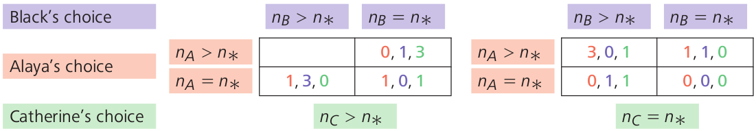
*Figure 1.* The payoffs to the players in the game when $n_{*} < \infty$ . In red, purple, and green the choices and payoffs of respectively Alaya, Black, and Catherine. Alaya chooses a row, Black a column, and Catherine a matrix.

Each entry in the figure represents one possible outcome. For example, when $n_{*} = n_{A} = n_{B} < n_{C}$ , the payoffs of the three players are $(1, 0, 1)$ : the left-most number in each entry is the payoff to Alaya, the middle number is the payoff to Black, and the right-most number is the payoff to Catherine. This game is an instance of a class of games that are known as quitting games.

How should the players act in this game? To provide an answer, we formalize the concepts of strategy and equilibrium. As the choice of each participant may be random, a strategy for a player is a probability distribution over $N \cup {\infty}$ . Denote a strategy of Alaya (resp. Black, Catherine) by $σ_{A}$ (resp. $σ_{B}$ , $σ_{C}$ ), and by $γ_{i} (σ_{A}, σ_{B}, σ_{C})$ the expected payoff to player $i$ under the vector of strategies $(σ_{A}, σ_{B}, σ_{C})$ . A vector of strategies $(σ_{A}^{*}, σ_{B}^{*}, σ_{C}^{*})$ is an equilibrium if no player can increase her or his expected payoff by adopting another strategy while the other two stick to their strategies:

γ_{A} (σ_{A}^{*}, σ_{B}^{*}, σ_{C}^{*}) \geq γ_{A} (σ_{A}, σ_{B}^{*}, σ_{C}^{*})

for every strategy $σ_{A}$ of Alaya, and analogous inequalities hold for Black and Catherine.

The three-player quitting game with payoffs as described above was studied by Flesch, Thuijsman, and Vrieze [⁠15⁠ J. Flesch, F. Thuijsman and K. Vrieze, Cyclic Markov equilibria in stochastic games. Internat. J. Game Theory26, 303–314 (1997) ] who proved that the following vector of strategies $(σ_{A}^{*}, σ_{B}^{*}, σ_{C}^{*})$ is an equilibrium:

σ_{A}^{*} : σ_{B}^{*} : σ_{C}^{*} : 1 \frac{1}{2} 00 20 \frac{1}{2} 0 300 \frac{1}{2} 4 \frac{1}{4} 00 50 \frac{1}{4} 0 600 \frac{1}{4} 7 \frac{1}{8} 00 80 \frac{1}{8} 0 900 \frac{1}{8} \dots \dots \dots \dots \infty 000

Under $(σ_{A}^{*}, σ_{B}^{*}, σ_{C}^{*})$ , with probability 1 the minimum $n_{*}$ is the choice of exactly one player: $n_{*} = n_{A}$ with probability $\frac{4}{7}$ , $n_{*} = n_{B}$ with probability $\frac{2}{7}$ , and $n_{*} = n_{C}$ with probability $\frac{1}{7}$ . It follows that the vector of expected payoffs under $(σ_{A}^{*}, σ_{B}^{*}, σ_{C}^{*})$ is

γ (σ_{A}^{*}, σ_{B}^{*}, σ_{C}^{*}) = \frac{4}{7} \cdot (1, 3, 0) + \frac{2}{7} \cdot (0, 1, 3) + \frac{1}{7} \cdot (3, 0, 1) = (1, 2, 1) .

Can a player profit by adopting a strategy different than $σ_{A}^{*}$ , $σ_{B}^{*}$ , or $σ_{C}^{*}$ , assuming the other two stick to their prescribed strategies? It is a bit tedious, but not too difficult, to verify that this is not the case, hence $(σ_{A}^{*}, σ_{B}^{*}, σ_{C}^{*})$ is indeed an equilibrium.

In fact, Flesch, Thuijsman, and Vrieze [⁠15⁠ J. Flesch, F. Thuijsman and K. Vrieze, Cyclic Markov equilibria in stochastic games. Internat. J. Game Theory26, 303–314 (1997) ] proved that under all equilibria of the game, with probability 1 the minimum $n_{*}$ coincides with the choice of exactly one player. Moreover, a vector of strategies is an equilibrium if and only if the set $N$ can be partitioned into blocks of consecutive numbers, and up to circular permutations of the players, the support of the strategy of Alaya (which is a probability distribution over $N \cup {\infty}$ ) is contained in blocks number $1, 4, 7, \dots$ , and the total probability that $n_{A}$ is in block $3 k - 2$ is $\frac{1}{2 ^{k}}$ (for each $k \in N$ ), the support of the strategy of Black (resp. Catherine) is contained in blocks number $2, 5, 8, \dots$ (resp. $3, 6, 9, \dots$ ), and the total probability that $n_{B}$ (resp. $n_{C}$ ) is in block $3 k - 1$ (resp. $3 k$ ) is $\frac{1}{2 ^{k}}$ (for each $k \in N$ ).

Does an equilibrium exist if the payoffs are not given by the table in Figure ⁠1⁠, but rather by other numbers? Solan [⁠19⁠ E. Solan, The dynamics of the Nash correspondence and n-player stochastic games. Int. Game Theory Rev.3, 291–299 (2001) ] showed that this is not the case. He studied a three-player quitting game that differs from the game of [⁠15⁠ J. Flesch, F. Thuijsman and K. Vrieze, Cyclic Markov equilibria in stochastic games. Internat. J. Game Theory26, 303–314 (1997) ] in three payoffs:

the payoffs in the entry $n_{*} = n_{A} = n_{B} < n_{C}$ are $(1 + η, 0, 1)$ ,
the payoffs in the entry $n_{*} = n_{A} = n_{C} < n_{B}$ are $(0, 1, 1 + η)$ ,
the payoffs in the entry $n_{*} = n_{B} = n_{C} < n_{A}$ are $(1, 1 + η, 0)$ ;

and showed that provided $η$ is sufficiently small, the game has no equilibrium. For example, the strategy vector $(σ_{A}^{*}, σ_{B}^{*}, σ_{C}^{*})$ described above is no longer an equilibrium, because Catherine is better off selecting $n_{C} = 1$ with probability 1, thereby obtaining expected payoff $\frac{1}{2} \cdot 1 + \frac{1}{2} \cdot (1 + η) = 1 + \frac{η}{2}$ , which is higher than her expected payoff under $(σ_{A}^{*}, σ_{B}^{*}, σ_{C}^{*})$ (that is still 1).

Yet in Solan’s variation [⁠19⁠ E. Solan, The dynamics of the Nash correspondence and n-player stochastic games. Int. Game Theory Rev.3, 291–299 (2001) ], for every $ε > 0$ there is an $ε$ -equilibrium: a vector of strategies such that no player can profit more than $ε$ by deviating to another strategy, in other words,

γ_{A} (σ_{A}^{*}, σ_{B}^{*}, σ_{C}^{*}) \geq γ_{A} (σ_{A}, σ_{B}^{*}, σ_{C}^{*}) - ε,

for every strategy $σ_{A}$ of Alaya, and analogous inequalities hold for Black and Catherine. Indeed, given a positive integer $m$ , consider the following variation of $(σ_{A}^{*}, σ_{B}^{*}, σ_{C}^{*})$ , denoted $(\overset{σ}{^}_{A}, \overset{σ}{^}_{B}, \overset{σ}{^}_{C})$ , where the set $N$ is partitioned into blocks of size $m$ : block $k$ contains the integers ${(k - 1) m + 1, (k - 1) m + 2, \dots, km}$ , for each $k \in N$ . $\overset{σ}{^}_{A}$ is the probability distribution that assigns to each integer in block $3 k - 2$ the probability $\frac{1}{m \cdot 2 ^{k}}$ , for every $k \in N$ . Similarly, $\overset{σ}{^}_{B}$ (resp. $\overset{σ}{^}_{C}$ ) is the probability distribution that assigns to each integer in block $3 k - 1$ (resp. $3 k$ ) the probability $\frac{1}{m \cdot 2 ^{k}}$ , for every $k \in N$ . As mentioned above, the strategy vector $(\overset{σ}{^}_{A}, \overset{σ}{^}_{B}, \overset{σ}{^}_{C})$ is an equilibrium of the game whose payoff function is given in Figure ⁠1⁠, and one can verify that provided $m \geq \frac{1}{ε}$ , it is an $ε$ -equilibrium of Solan’s variation [⁠19⁠ E. Solan, The dynamics of the Nash correspondence and n-player stochastic games. Int. Game Theory Rev.3, 291–299 (2001) ].

It follows from [⁠18⁠ E. Solan, Three-player absorbing games. Math. Oper. Res.24, 669–698 (1999) ] that an $ε$ -equilibrium exists in every three-player quitting game, for every $ε > 0$ , regardless of the payoffs. One of the most challenging problems in game theory to date is the following.

251*

Does an $ε$ -equilibrium exist in quitting games that include more than three players, for every $ε > 0$ ?

For partial results, see [⁠21⁠E. Solan and N. Vieille, Quitting games. Math. Oper. Res.26, 265–285 (2001) , ⁠22⁠ E. Solan and N. Vieille, Quitting games – an example. Internat. J. Game Theory31, 365–381 (2002) , ⁠16⁠R. S. Simon, The structure of non-zero-sum stochastic games. Adv. in Appl. Math.38, 1–26 (2007) , ⁠17⁠ R. S. Simon, A topological approach to quitting games. Math. Oper. Res.37, 180–195 (2012) , ⁠20⁠ E. Solan and O. N. Solan, Quitting games and linear complementarity problems. Math. Oper. Res.45, 434–454 (2020) , ⁠14⁠ G. Ashkenazi-Golan, I. Krasikov, C. Rainer and E. Solan, Absorption paths and equilibria in quitting games. arXiv:2012.04369 (2021) ], which use different tools to study the problem: dynamical systems, algebraic topology, and linear complementarity problems. The open problem is a step in solving several other well-known open problems in game theory: the existence of $ε$ -equilibria in stopping games, the existence of uniform equilibria in stochastic games, and the existence of $ε$ -equilibria in repeated games with Borel-measurable payoffs.

It is interesting to note that if we defined

n_{*} : = max {1_{{n_{A} < \infty}} \cdot n_{A}, 1_{{n_{B} < \infty}} \cdot n_{B}, 1_{{n_{C} < \infty}} \cdot n_{C}},

then an $ε$ -equilibrium need not exist for small $ε > 0$ . Indeed, with this definition, the three-player game in which the payoff of player $i$ is 1 if $\infty > n_{i} = n_{*} > n_{j}$ for each $j \neq = i$ , and 0 otherwise, has no $ε$ -equilibrium for $ε \in (0, \frac{2}{3})$ .

III Solutions

237

We take for our probability space $(X, m)$ : the unit interval $X = [0, 1]$ equipped with Lebesgue measure $m$ defined on $B (X)$ , the Borel subsets of $X$ and let $(X, m, T)$ be an invertible measure preserving transformation, that is $T : X_{0} \to X_{0}$ is a bimeasurable bijection of some Borel set $X_{0} \in B (X)$ of full measure so that and $m (T A) = m (T^{- 1} A) = m (A)$ for every $A \in B (X)$ .

Suppose also that $T$ is ergodic in the sense that the only $T$ -invariant Borel sets have either zero- or full measure ( $A \in B (X)$ , $T A = A \Rightarrow m (A) = 0, 1$ ).

Birkhoff’s ergodic theorem says that for every integrable function $f : X \to R$ ,

\frac{1}{n} k = 0 \sum n - 1 f \circ T^{k} n \to \infty E (f) : = \int_{X} f d m a.s.

The present exercise is concerned with the possibility of generalizing this. Throughout, $(X, m, T)$ is an arbitrary ergodic, measure preserving transformation as above.

Warm-up 1. Show that if $f : X \to R$ is measurable, and

m ([n \to \infty \overline{lim} k = 0 \sum n - 1 f \circ T^{k} < \infty]) > 0,

then $\frac{1}{n} \sum_{k = 0}^{n - 1} f \circ T^{k}$ converges in $R$ a.s.

Warm-up 1 is [⁠23⁠ P. Hagelstein, D. Herden and A. Stokolos, A theorem of Besicovitch and a generalization of the Birkhoff ergodic theorem. Proc. Amer. Math. Soc. Ser. B8, 52–59 (2021) , Lemma 1]. For a multidimensional version, see [⁠23⁠ P. Hagelstein, D. Herden and A. Stokolos, A theorem of Besicovitch and a generalization of the Birkhoff ergodic theorem. Proc. Amer. Math. Soc. Ser. B8, 52–59 (2021) , Conjecture 3].

Warm-up 2. Show that if $f : X \to R$ is as in Warm-up 1, there exist $g, h : X \to R$ measurable with $h$ bounded so that $f = h + g - g \circ T^{n}$ .

Warm-up 2 is established by adapting the proof of [⁠25⁠ D. Volný and B. Weiss, Coboundaries in L0∞. Ann. Inst. H. Poincaré Probab. Statist.40, 771–778 (2004) , Theorem A].

Problem. Show that there is a measurable function $f : X \to R$ satisfying $E (∣ f ∣) = \infty$ so that

\frac{1}{n} k = 0 \sum n - 1 f \circ T^{k}

converges in $R$ a.s.

The existence of such $f$ for a specially constructed ergodic measure preserving transformation is shown in [⁠24⁠ D. Tanny, A zero-one law for stationary sequences. Z. Wahrscheinlichkeitstheorie und Verw. Gebiete30, 139–148 (1974) , Example b]. The point here is to prove it for an arbitrary ergodic measure preserving transformation of $(X, m)$ .

Jon Aaronson (Tel Aviv University, Israel)

Solution by the proposer

We’ll fix sequences $ε_{k}, M_{k} > 0$ , $N_{k} \in N$ ( $k \geq 1$ ). For each $ε, M > 0$ , $N \geq 1$ , we’ll construct a small coboundary $f^{(ε, M, N)}$ . The desired function will be of the form $F : = \sum_{k \geq 1} f^{(ε_{k}, M_{k}, N_{k})}$ for a suitable choice of $ε_{k}, M_{k} > 0$ , $N_{k} \in N$ ( $k \geq 1$ ).

To construct $f^{(ε, M, N)}$ , choose, using Rokhlin’s lemma, a set $B \in B$ such that ${T^{k} B : ∣ k ∣ \leq 2 N}$ are disjoint and $m (A) = ε$ where $A : = ⨃_{∣ k ∣ \leq 2 N} T^{k} B$ . Let

f = f^{(ε, M, N)} : = M k = 1 \sum 2 N (- 1)^{k} 1_{T_{k} B} .

It follows that

S_{n} f (x) \in {0, M, - M} for all n \geq 1, x \in X;

S_{n} f (x) = 0 for all 1 \leq n \leq N, x \in / A;

E (∣ f ∣) = M m (⨃_{j = 1}^{2 N} T^{j} B) = \frac{Mε 2 N}{4 N + 1} > \frac{Mε}{3} .

Set $ε_{k} : = \frac{1}{5 ^{k}}$ , $M_{k} = 6^{k}$ , $N_{k} = 7^{k}$ , and define $F^{(k)} : = f^{(ε_{k}, M_{k}, N_{k})}$ as above.

Since

k \geq 1 \sum m ([F^{(k)} \neq = 0]) \leq k \geq 1 \sum ε_{k} < \infty,

this is a finite sum and so

F : = k \geq 1 \sum F^{(k)} : X \to R .

Proof that $E (∣ F ∣) = \infty$ . For each $K \geq 1$ ,

∣ F ∣ \geq F^{(K)} + 1 \leq j \leq K - 1 \sum F^{(j)} 1_{[F^{(k)} = 0 \forall k > K]} \geq (∣ F^{(K)} ∣ - 1 \leq j \leq K - 1 \sum ∣ F^{(j)} ∣) 1_{[F^{(k)} = 0 \forall k > K]} \geq (M_{K} - 1 \leq j \leq K - 1 \sum M_{j}) 1_{[F^{(K)} \neq = 0 & F^{(k)} = 0 \forall k > K]} \geq \frac{4}{5} M_{K} 1_{[F^{(K)} \neq = 0 & F^{(k)} = 0 \forall k > K]}

and

E (∣ F ∣) \geq \frac{4}{5} M_{K} m ([F^{(K)} \neq = 0 & F^{(k)} = 0 \forall k > K]) .

Next,

E_{K} : = [F^{(k)} = 0 \forall k > K]^{c} = k \geq K + 1 ⋃ 1 \leq j \leq 2 N_{k} ⋃ T^{k} B_{k}

whence

m (E_{K}) \leq k \geq K + 1 \sum \frac{ε _{k}}{2} = \frac{1}{2} k \geq K + 1 \sum \frac{1}{5 ^{k}} = \frac{ε _{K}}{40} .

It follows that

m ([F^{(K)} \neq = 0] ∖ E_{K}) = m (⨃_{j = 1}^{2 N_{K}} T^{j} B_{K} ∖ E_{K}) > \frac{ε _{K}}{3} - \frac{ε _{K}}{40} = \frac{37 ε _{K}}{120},

whence

E (∣ F ∣) \geq \frac{4}{5} M_{K} m ([F^{(K)} \neq = 0] ∖ E_{K}) > \frac{37 ε _{K} M _{K}}{150} K \to \infty \infty.

∎

Proof that $S_{n} F = o (n)$ a.s.. There is a function $κ : X \to N$ so that for a.s. $x \in X$ , $x \in A_{k}^{c}$ for all $k \geq κ (x)$ . Suppose that $k \geq κ (x)$ and $2 N_{k} \leq n < 2 N_{k + 1}$ , then

∣ S_{n} F (x)∣ = j = 1 \sum k S_{n} F^{(j)} (x) \leq j = 1 \sum k M_{j} < \frac{6}{5} \cdot (\frac{6}{7})^{k} \cdot N_{k}

and

\frac{∣ S _{n} F ( x )∣}{n} n \to \infty 0 a.s.

∎

238

Let $(Ω, F, P)$ be a probability space and ${X_{n} : n \geq 1}$ be a sequence of independent and identically distributed (i.i.d.) random variables on $Ω$ . Assume that there exists a sequence of positive numbers ${b_{n} : n \geq 1}$ such that $\frac{b _{n}}{n} \leq \frac{b _{n + 1}}{n + 1}$ for every $n \geq 1$ , $lim_{n \to \infty} \frac{b _{n}}{n} = \infty$ , and $\sum_{n = 1}^{\infty} P (∣ X_{n} ∣ \geq b_{n}) < \infty$ . Prove that, if $S_{n} : = \sum_{j = 1}^{n} X_{j}$ for each $n \geq 1$ , then

n \to \infty lim \frac{S _{n}}{b _{n}} = 0 almost surely .

Comment. The desired statement says that, if such a sequence ${b_{n} : n \geq 1}$ exists, then ${X_{n} : n \geq 1}$ satisfies the (generalized) Strong Law of Large Numbers (SLLN) when averaged by ${b_{n} : n \geq 1}$ . If $X_{n} \in L^{1} (P)$ for every $n \geq 1$ , then the desired statement follows trivially from Kolmogorov’s SLLN, since in which case, with probability one,

n \to \infty lim \frac{S _{n}}{n} = E [X_{1}],

and hence

\frac{S _{n}}{b _{n}} = \frac{S _{n}}{n} \cdot \frac{n}{b _{n}}

must converge to 0 under the assumptions on ${b_{n} : n \geq 1}$ . Therefore, the desired statement can be viewed as an alternative to Kolmogorov’s SLLN for i.i.d. random variables that are not integrable.

Linan Chen (McGill University, Montreal, Quebec, Canada)

Solution by the proposer

As explained above, we will need to prove the desired statement without assuming integrability of $X_{n}$ ’s. For every $n \geq 1$ , we truncate $X_{n}$ at the level $b_{n}$ by defining $Y_{n} = X_{n}$ if $∣ X_{n} ∣ < b_{n}$ , and $Y_{n} = 0$ if $∣ X_{n} ∣ \geq b_{n}$ . Then, ${Y_{n} : n \geq 1}$ is again a sequence of independent random variables. It follows from the assumption on ${b_{n} : n \geq 1}$ that

n = 1 \sum \infty P (X_{n} \neq = Y_{n}) = n = 1 \sum \infty P (∣ X_{n} ∣ \geq b_{n}) < \infty,

which, by the Borel–Cantelli lemma, implies that the sequence of the truncated random variables ${Y_{n} : n \geq 1}$ is equivalent to the original sequence ${X_{n} : n \geq 1}$ in the sense that

P (X_{n} \neq = Y_{n} infinitely often) = 0, or equivalently,

P (X_{n} = Y_{n} eventually always) = 1.

Next, by setting $b_{0} = 0$ , we have that

n = 1 \sum \infty P (∣ X_{n} ∣ \geq b_{n}) = n = 1 k \sum \infty k = n + 1 \sum \infty P (b_{k - 1} \leq ∣ X_{1} ∣ < b_{k}) = k = 2 \sum \infty n = 1 k \sum k - 1 P (b_{k - 1} \leq ∣ X_{1} ∣ < b_{k}) = k = 2 \sum \infty (k - 1) P (b_{k - 1} \leq ∣ X_{1} ∣ < b_{k}) = k = 1 \sum \infty k P (b_{k - 1} \leq ∣ X_{1} ∣ < b_{k}) - 1,

and hence the assumption on ${b_{n} : n \geq 1}$ implies that

k = 1 \sum \infty k P (b_{k - 1} \leq ∣ X_{1} ∣ < b_{k}) < \infty.

Our next goal is to establish the desired SLLN statement for ${Y_{n} : n \geq 1}$ . To be specific, we want to show that if $T_{n} : = \sum_{j = 1}^{n} Y_{j}$ for each $n \geq 1$ , then $lim_{n \to \infty} \frac{T _{n}}{b _{n}} = 0$ almost surely. We will achieve this goal in two steps.

Step 1 is to treat the convergence of $\frac{E [ T _{n} ]}{b _{n}}$ . To this end, we derive an upper bound for this term as

\frac{E [∣ T _{n} ∣]}{b _{n}} \leq \frac{1}{b _{n}} j = 1 \sum n E [∣ Y_{j} ∣] = \frac{1}{b _{n}} j = 1 \sum n \int_{{∣ X_{1} ∣ < b_{j}}} ∣ X_{1} ∣ d P = \frac{1}{b _{n}} j = 1 k \sum n k = 1 \sum j \int_{{b_{k - 1} \leq ∣ X_{1} ∣ < b_{k}}} ∣ X_{1} ∣ d P \leq \frac{1}{b _{n}} k = 1 \sum n (n - k + 1) b_{k} P (b_{k - 1} \leq ∣ X_{1} ∣ < b_{k}) \leq \frac{2 n}{b _{n}} k = 1 \sum n b_{k} P (b_{k - 1} \leq ∣ X_{1} ∣ < b_{k}) .

Then (⁠2⁠) implies that

k = 1 \sum \infty \frac{b _{k} P ( b _{k - 1} \leq ∣ X _{1} ∣ < b _{k} )}{( b _{k} / k )} = k = 1 \sum \infty k P (b_{k - 1} \leq ∣ X_{1} ∣ < b_{k}) < \infty,

which, by Kronecker’s lemma, leads to

n \to \infty lim \frac{n}{b _{n}} k = 1 \sum n b_{k} P (b_{k - 1} \leq ∣ X_{1} ∣ < b_{k}) = 0.

Hence, we conclude that $lim_{n \to \infty} \frac{E [∣ T _{n} ∣]}{b _{n}} = 0$ .

Step 2 is to establish the convergence of $\frac{T _{n} - E [ T _{n} ]}{b _{n}}$ , for which we will use a martingale convergence argument. We note that if

M_{n} : = j = 1 \sum n \frac{Y _{j} - E [ Y _{j} ]}{b _{j}}

for each $n \geq 1$ , then ${M_{n} : n \geq 1}$ is a martingale (with respect to the natural filtration) and for each $n \geq 1$ ,

E [M_{n}^{2}] \leq j = 1 \sum n \frac{E [ Y _{j}^{2} ]}{b _{j}^{2}} = j = 1 \sum n \frac{1}{b _{j}^{2}} \int_{{∣ X_{1} ∣ < b_{j}}} X_{1}^{2} d P \leq j = 1 k \sum n k = 1 \sum j \frac{b _{k}^{2}}{b _{j}^{2}} P (b_{k - 1} \leq ∣ X_{1} ∣ < b_{k}) \leq k = 1 \sum n (j = k \sum n \frac{1}{j ^{2}}) k^{2} P (b_{k - 1} \leq ∣ X_{1} ∣ < b_{k}) \leq C k = 1 \sum n k P (b_{k - 1} \leq ∣ X_{1} ∣ < b_{k}),

where the second last inequality follows from the assumption that $\frac{b _{n}}{n}$ is increasing in $n$ , and the last inequality is due to the fact that there exists constant $C > 0$ such that $\sum_{j = k}^{\infty} \frac{1}{j ^{2}} \leq \frac{C}{k}$ for every $k \geq 1$ . Hence, (⁠2⁠) implies that ${M_{n} : n \geq 1}$ is bounded in $L^{2} (P)$ . A standard martingale convergence result implies that $lim_{n \to \infty} M_{n}$ exists in $R$ almost surely⁠³⁠One can also use Kolmogorov’s maximal inequality to prove the almost sure existence of the limit of $M_{n}$ ., which, by Kronecker’s lemma again, leads to

n \to \infty lim \frac{T _{n} - E [ T _{n} ]}{b _{n}} = 0 almost surely .

Finally, we write $\frac{S _{n}}{b _{n}}$ as

\frac{S _{n}}{b _{n}} = \frac{S _{n} - T _{n}}{b _{n}} + \frac{T _{n} - E [ T _{n} ]}{b _{n}} + \frac{E [ T _{n} ]}{b _{n}},

where the last two terms have been proven to converge to 0 almost surely, and (⁠1⁠) implies that, with probability one, the limit of the first term is also 0. We have completed the proof.

239

In Beetown, the bees have a strict rule: all clubs must have exactly $k$ members. Clubs are not necessarily disjoint. Let $b (k)$ be the smallest number of clubs that the $n \geq k^{2}$ bees can form, such that no matter how they divide themselves into two teams to play beeball, there will always be a club all of whose membees are on the same team. Prove that

2^{k - 1} \leq b (k) \leq C k^{2} \cdot 2^{k}

for some constant $C > 0$ .

Rob Morris (IMPA, Rio de Janeiro, Brasil)

Solution by the proposer

This is an old result of Erdős, and a classic application of the probabilistic method. Let us think of the two teams as being red and blue, so that a club is ‘monochromatic’ if all of its membees are on the same team.

First, for the lower bound, we need to show that if $m < 2^{k - 1}$ , then for any collection of $m$ clubs there exists a colouring with no monochromatic club. To do so, we choose the teams randomly, and observe that the expected number of monochromatic clubs is less than $1$ . To be precise, let $Pr (b is red) = \frac{1}{2}$ , independently for each bee $b$ , and let $S$ count the number of monochromatic clubs. Then, by linearity of expectation, $E [S] = m \cdot 2^{- k + 1} < 1$ , since each club is monochromatic with probability exactly $2^{- k + 1}$ . But this implies that $Pr (S = 0) > 0$ , so there exists a colouring with no monochromatic club, as required.

For the upper bound, we choose the clubs randomly. To be precise, choose $N = k^{2}$ bees, and choose each club uniformly and independently from the $k$ -subsets of these $N$ bees. The idea is that, for any colouring of the bees, the expected number of monochromatic clubs is at least $k^{2}$ , so the probability of having no monochromatic club should be at most $e^{- k^{2}}$ . Since there are $2^{k^{2}}$ colourings of these bees, the expected number of colourings with no monochromatic clubs is less than $1$ , so there must exist a choice for which it is zero.

To spell out the details, fix a colouring, and suppose that $x$ of the $N$ chosen bees are red. The probability that a random club is monochromatic is

((k x) + (k N - x)) (k N)^{- 1} \geq 2 \cdot (k N /2) (k N)^{- 1} \geq 2^{- k - c}

for some constant $c > 0$ , where in the final inequality we used the fact that $N \geq k^{2}$ .

Now, let $T$ count the number of colourings of the $N$ bees with no monochromatic club, and observe that if there are $m = k^{2} 2^{k + c}$ clubs, then

E [T] \leq colourings of the N bees \sum (1 - 2^{- k - c})^{m} \leq 2^{k^{2}} e^{- k^{2}} < 1.

It follows that there exists a choice of $m$ clubs such that $T = 0$ , as required.

240

$N$ agents are in a room with a server, and each agent is looking to get served, at which point the agent leaves the room. At any discrete time step, each agent may choose to either shout or stay quiet, and an agent gets served in that round if (and only if) that agent is the only one to have shouted. The agents are indistinguishable to each other at the start, but at each subsequent step, every agent gets to see who has shouted and who has not. If all the agents are required to use the same randomised strategy, show that the minimum time to clear the room in expectation is $N + (2 + o (1)) lo g_{2} N$ .

Bhargav Narayanan (Rutgers University, Piscataway, USA)

Solution by the proposer

Here is a simple strategy that works in expected time $N + (2 + o (1)) lo g_{2} N$ . The agents all toss independent fair coins to decide whether to shout or not in each of the first $k = (2 + o (1)) lo g_{2} N$ rounds. It is easy to see that with high probability, after these $k$ rounds, every agent (still in the room) has a unique ‘history’, i.e. no two agents have the exact same sequence of turns (shouting/staying quiet). Now the agents are all distinguishable, and we are done in $N$ more steps; for example, the agents can interpret each others histories as numbers in binary, and can get served in increasing order. Below, we show that no strategy can do significantly better.

At any time, we can partition all the agents into clusters based on their history so far: two agents go into the same cluster if they have chosen to do the same thing in all previous rounds. By the requirement that the agents all have the same randomised strategy, we know that at any time, all the agents in the same cluster must have the same strategy. Let $X$ be the number of times an agent from a cluster of size at least 2 gets served and leaves the room, and let $Y$ be the number of times either

exactly two agents from the same cluster, and nobody else, ask to be served, or
nobody asks to be served at all.

An easy computation shows that

P (Bin (m, p) = 1) \leq P (Bin (m, p) = 0) + P (Bin (m, p) = 2)

for all $m > 1$ and any $0 \leq p \leq 1$ ; consequently, it is easy to see that $Y$ stochastically dominates $X$ . So, if for some strategy,

P (X > 2 (lo g_{2} N)^{2}) > \frac{1}{lo g _{2} N},

then the expected time to clear the room, which is at least $N + Y$ , is at least $N + 2 lo g_{2} N$ in expectation. So we may assume that $X < 2 (lo g_{2} N)^{2}$ with high probability for any strategy under consideration.

Let $S$ be the set of agents who leave the room only when they belong to their own singleton cluster. As we just observed, the number of such agents $∣ S ∣ = M = N - X$ may be assumed to be at least $N - 2 (lo g_{2} N)^{2}$ . The key observation is this: if someone leaves the room in a particular step, the cluster structure of $S$ does not change in that step. To see this, note that when an agent not from $S$ leaves the room, that agent shouts and everyone in $S$ does not, so there is no change to the cluster structure of $S$ . On the other hand, when an agent from $S$ leaves the room, that agent is, by definition, already in their own singleton cluster, and every other agent in $S$ does not shout in this step; again, there is no change in the cluster structure of $S$ .

But we know that at the end of the process, which let us say takes $N + Δ$ rounds, $S$ has been split from a single cluster into $M$ singleton clusters. Nothing changes in the cluster structure of $S$ in the $N$ rounds when someone leaves the room, so $S$ gets broken down into singleton clusters in the remaining $Δ$ steps.

Consider these $Δ$ steps where nobody leaves the room. Deterministically, in the first $lo g_{2} M - 1$ of these steps, we can produce at most $\frac{M}{2}$ singletons in $S$ . The remaining $\frac{M}{2}$ agents in $S$ are all in clusters of size at least 2. Divide all these cluster into sub-clusters each of size 2 (by ignoring agents if necessary). The result is at least $\frac{M}{6}$ 2-clusters that we still need to break down into singletons (the worst case being when the $\frac{M}{2}$ agents are each in a cluster of size 3). The probability that a 2-cluster breaks down into two singletons at any given time step, with any strategy, is at most $\frac{1}{2}$ . So in any strategy, we need at least another $lo g_{2} M - lo g_{2} lo g_{2} M$ time steps, say, for all these 2-clusters to separate into singletons. Thus, $Δ \geq 2 lo g_{2} M - lo g_{2} lo g_{2} M$ with high probability, which with our previous bound on $M$ , tells us that any strategy takes at least $N + (2 - o (1)) lo g_{2} N$ steps to clear the room.

241

Consider the following sequence of partitions of the unit interval $I$ : First, define $π_{1}$ to be the partition of $I$ into two intervals, a red interval of length $\frac{1}{3}$ and a blue one of length $\frac{2}{3}$ . Next, for any $m > 1$ , define $π_{m + 1}$ to be the partition derived from $π_{m}$ by splitting all intervals of maximal length in $π_{m}$ , each into two intervals, a red one of ratio $\frac{1}{3}$ and a blue one of ratio $\frac{2}{3}$ , just as in the first step. For example $π_{2}$ consists of three intervals of lengths $\frac{1}{3}$ (red), $\frac{2}{9}$ (red) and $\frac{4}{9}$ (blue), the last two are the result of splitting the blue interval in $π_{1}$ . The figure above illustrates $π_{1}, \dots, π_{4}$ , from top to bottom.

🅭🅯 CC BY 4.0

Let $m \in N$ and consider the $m$ -th partition $π_{m}$ .

Choose an interval in $π_{m}$ uniformly at random. Let $R_{m}$ be the probability you chose a red interval. Does the sequence $(R_{m})_{m \in N}$ converge? If so, what is the limit?
Choose a point in $I$ uniformly at random. Let $A_{m}$ be the probability that the point is colored red. Does the sequence $(A_{m})_{m \in N}$ converge? If so, what is the limit?

Yotam Smilansky (Rutgers University, NJ, USA)

Solution by the proposer

The proposed solution is based on path counting results [⁠26⁠ A. Kiro, Y. Smilansky and U. Smilansky, The distribution of path lengths on directed weighted graphs. In Analysis as a Tool in Mathematical Physics, Oper. Theory Adv. Appl. 276, Birkhäuser/Springer, Cham, 351–372 (2020) ] on an appropriately defined graph, and can be generalized to higher dimensions and to more complicated sequences of partitions [⁠27⁠ Y. Smilansky, Uniform distribution of Kakutani partitions generated by substitution schemes. Israel J. Math.240, 667–710 (2020) ].

Let $G$ be a weighted graph with a single vertex and two directed loops: a red one of length $- lo g (\frac{1}{3})$ and a blue one of length $- lo g (\frac{2}{3})$ , and consider directed walks along the edges of $G$ that originate at the vertex and terminate on a point of a colored loop. The first important observation is that there is a 1-1 correspondence between colored intervals in $π_{m}$ and walks of length $ℓ_{m}$ on $G$ , where $(ℓ_{m})_{m \in N}$ is the increasing sequence of lengths of closed orbits on $G$ . In the following illustration, the top is partition $π_{1}$ and the corresponding two walks of length $ℓ_{1} = - lo g (\frac{2}{3})$ , and the bottom is partition $π_{2}$ and the corresponding three walks of length $ℓ_{2} = - 2 lo g (\frac{2}{3})$ .

🅭🅯 CC BY 4.0

In general, a splitting of an interval corresponds to an extension of a walk that terminates at the vertex to two new walks, one that extends onto the red loop and the other onto the blue. Therefore, $R_{m}$ is the relative part of walks of length $ℓ_{m}$ that terminate on the red loop. For $A_{m}$ , consider random walks on $G$ and prescribe probabilities to the two outgoing loops: a walk along $G$ is extended onto the red loop when reaching the vertex with probability $\frac{1}{3}$ , and onto the blue loop with probability $\frac{2}{3}$ . These are chosen because $\frac{1}{3}$ of a split interval is colored red and $\frac{2}{3}$ colored blue. It follows that $A_{m}$ is the probability that a walker is located on the red loop after walking a walk of length $ℓ_{m}$ .

The second observation is that in order to compute the asymptotic behavior of $R_{m}$ and $A_{m}$ , one can apply the well-known Wiener–Ikehara theorem, originally devised to approach the prime number theorem. The theorem states that if there exists $λ \in R$ for which the Laplace transform of a counting function is analytic for $ℜ (s) > λ$ , has a simple pole at $s = λ$ and no other singular points on the vertical line $ℜ (s) = λ$ , then the main term of the growth rate is $c e^{λ x}$ , with $c$ the residue of the Laplace transform at $s = λ$ .

A direct computation shows that the Laplace transform for the number of walks that terminate on the red loop is

\frac{1}{s} \cdot \frac{1 - ( \frac{1}{3} ) ^{s}}{1 - ( \frac{1}{3} ) ^{s} - ( \frac{2}{3} ) ^{s}} .

Inspecting the term $1 - (\frac{1}{3})^{s} - (\frac{2}{3})^{s}$ one sees that $s = 1$ is a simple root of maximal real part, and so to apply the Wiener–Ikehara theorem it suffices to establish that there are no other roots of the form $1 + i t$ . Indeed, a careful but elementary inspection shows that otherwise, the loops of $G$ must have commensurable lengths, or equivalently $lo g_{2} 3 \in Q$ , which is of course false. The Laplace transform of the total number of walks is similar but has numerator $2 - (\frac{1}{3})^{s} - (\frac{2}{3})^{s}$ , and so $R_{m}$ tends to the ratio of the residues of these two transforms at $s = 1$ , that is, $lim_{m \to \infty} R_{m} = \frac{2}{3}$ . Similarly, the Laplace transform for $A_{m}$ is

\frac{\frac{1}{3}}{s} \cdot \frac{1 - ( \frac{1}{3} ) ^{s}}{1 - ( \frac{1}{3} ) ^{s + 1} - ( \frac{2}{3} ) ^{s + 1}},

with the same poles but shifted by $- 1$ . It follows that $A_{m}$ converges to the residue at $s = 0$ , namely

m \to \infty lim A_{m} = \frac{- \frac{1}{3} lo g \frac{1}{3}}{- \frac{1}{3} lo g \frac{1}{3} - \frac{2}{3} lo g \frac{2}{3}} .

Note that the limit of $R_{m}$ is simply the length of the blue interval in $π_{1}$ , and the limit of $A_{m}$ can be viewed as the relative contribution of the red interval to the partition entropy of $π_{1}$ . This interpretation leads me to suspect that there may exist a more direct and illuminating approach to these problems, possibly based on tools from probability and dynamics, and I would be very happy to discuss any ideas or suggestions.

242

Prove that there exist $c < 1$ and $ε > 0$ such that if $A_{1}, \dots, A_{k}$ are increasing events of independent boolean random variables with $Pr (A_{i}) < ε$ for all $i$ , then

Pr (exactly one of A_{1}, \dots, A_{k} occurs) \leq c .

(What is the smallest $c$ that you can prove?)

Here $A \subset {0, 1}^{n}$ is an “increasing event” if whenever $x \in A$ , then the vector obtained by changing any coordinates of $x$ from $0$ to $1$ still lies in $A$ .

A useful fact is the Harris inequality, which states that for increasing events $A$ and $B$ of boolean random variables, $Pr (A \cap B) \geq Pr (A) Pr (B)$ .

I learned of this problem from Jeff Kahn.

Yufei Zhao (MIT, Cambridge, USA)

Solution by the proposer

We will show that the claim is true for every $ε > 0$ and $c = \frac{1 + ε}{2}$ .

If $Pr (A_{1} \cup \dots \cup A_{k}) \leq c$ , then the conclusion is automatic. So let us assume that $Pr (A_{1} \cup \dots \cup A_{k}) > c$ . Since $Pr (A_{i}) < ε$ for each $i$ , there exists some $j$ such that $Pr (A_{1} \cup \dots \cup A_{j})$ lies within $\frac{ε}{2}$ of $\frac{1}{2}$ . Let $B = A_{1} \cup \dots \cup A_{j}$ and $C = A_{j + 1} \cup \dots \cup A_{k}$ . We write $\overline{B}$ and $\overline{C}$ for the complementary events.

If exactly one of $A_{1}, \dots, A_{k}$ occurs, then exactly one of $B$ and $C$ can occur. So

Pr (exactly one of A_{1}, \dots, A_{k} occurs) \leq Pr (B \cap \overline{C}) + Pr (\overline{B} \cap C) \leq Pr (B) Pr (\overline{C}) + Pr (\overline{B}) Pr (C) \leq max {Pr (B), Pr (\overline{B})} \leq \frac{1 + ε}{2}

where the second inequality is due to Harris’ inequality.

Remark. It is conjectured that for any $c > \frac{1}{e}$ there exists some $ε > 0$ for which the statement is true. Here $\frac{1}{e}$ is optimal, since if $A_{i}$ are independent Bernoulli random variables with mean $\frac{1}{k}$ , then the number of occurrences is asymptotically Poisson with mean 1, with so that the probability of single occurrence is $\frac{1}{e} + o (1)$ .

We are eager to receive your solutions to the proposed problems, and any ideas that you may have on open problems. Send your solutions to Michael Th. Rassias (Institute of Mathematics, University of Zürich, Winterthurerstrasse 190, 8057 Zürich, Switzerland; michail.rassias@math.uzh.ch).

We also solicit your suggestions for new problems together with their solutions, for the next “Solved and unsolved problems” column, which will be devoted to Topology/Geometry.

¹
That is, a point such that each $x_{i, S} \in {0, 1}$ .
²
The author thanks János Flesch, Ehud Lehrer, and Abraham Neyman for commenting on earlier versions of the text, and acknowledges the support of the Israel Science Foundation, Grant #217/17.
³
One can also use Kolmogorov’s maximal inequality to prove the almost sure existence of the limit of $M_{n}$ .

References

V. Conitzer, Eliciting single-peaked preferences using comparison queries. J. Artificial Intelligence Res.35, 161–191 (2009)
C. H. Coombs. Psychological scaling without a unit of measurement. Psychological Review57, 145 (1950)
E. Elkind, M. Lackner and D. Peters. Structured preferences. In Trends in Computational Social Choice, edited by U. Endriss, Chapter 10, AI Access, 187–207 (2017)
H. Moulin, Axioms of Cooperative Decision Making. Cambridge University Press, Cambridge (1991)
T. Walsh, Generating single peaked votes. arXiv:1503.02766 (2015)
B. Cooper and C. Wallace, Group selection and the evolution of altruism. Oxford Economic Papers56, 307–330 (2004)
R. Povey, Punishment and the potency of group selection, J. Evolutionary Economics24 (2014)
G. R. Price, Selection and covariance, Nature227, 520–521 (1970)
G. R. Price, Extension of covariance selection mathematics, Ann. Human Genetics35, 485–490 (1972)
E. Sober and D. S. Wilson, Unto Others, Harvard University Press, Cambridge, Massachusetts (1999)
C. Ballester, A. Calvó-Armengol and Y. Zenou, Who’s who in networks. Wanted: the key player. Econometrica74, 1403–1417 (2006)
M. O. Jackson and Y. Zenou, Games on networks. In Handbook of Game Theory. Vol. 4, edited by H. P. Young and S. Zamir, Handbooks in Economics, 91–157, Elsevier/North-Holland, Amsterdam (2015)
Y. Sun, W. Zhao and J. Zhou, Structural interventions in networks. arXiv:2101.12420 (2021)
G. Ashkenazi-Golan, I. Krasikov, C. Rainer and E. Solan, Absorption paths and equilibria in quitting games. arXiv:2012.04369 (2021)
J. Flesch, F. Thuijsman and K. Vrieze, Cyclic Markov equilibria in stochastic games. Internat. J. Game Theory26, 303–314 (1997)
R. S. Simon, The structure of non-zero-sum stochastic games. Adv. in Appl. Math.38, 1–26 (2007)
R. S. Simon, A topological approach to quitting games. Math. Oper. Res.37, 180–195 (2012)
E. Solan, Three-player absorbing games. Math. Oper. Res.24, 669–698 (1999)
E. Solan, The dynamics of the Nash correspondence and n-player stochastic games. Int. Game Theory Rev.3, 291–299 (2001)
E. Solan and O. N. Solan, Quitting games and linear complementarity problems. Math. Oper. Res.45, 434–454 (2020)
E. Solan and N. Vieille, Quitting games. Math. Oper. Res.26, 265–285 (2001)
E. Solan and N. Vieille, Quitting games – an example. Internat. J. Game Theory31, 365–381 (2002)
P. Hagelstein, D. Herden and A. Stokolos, A theorem of Besicovitch and a generalization of the Birkhoff ergodic theorem. Proc. Amer. Math. Soc. Ser. B8, 52–59 (2021)
D. Tanny, A zero-one law for stationary sequences. Z. Wahrscheinlichkeitstheorie und Verw. Gebiete30, 139–148 (1974)
D. Volný and B. Weiss, Coboundaries in L0∞. Ann. Inst. H. Poincaré Probab. Statist.40, 771–778 (2004)
A. Kiro, Y. Smilansky and U. Smilansky, The distribution of path lengths on directed weighted graphs. In Analysis as a Tool in Mathematical Physics, Oper. Theory Adv. Appl. 276, Birkhäuser/Springer, Cham, 351–372 (2020)
Y. Smilansky, Uniform distribution of Kakutani partitions generated by substitution schemes. Israel J. Math.240, 667–710 (2020)

Cite this article

Michael Th. Rassias, Solved and unsolved problems. Eur. Math. Soc. Mag. 121 (2021), pp. 58–67

DOI 10.4171/MAG/38

🅭🅯

This open access article is published by EMS Press under a CC BY 4.0 license, with the exception of logos and branding of the European Mathematical Society and EMS Press, and where otherwise noted.

Back to Issue 121

[bib-bib1] V. Conitzer, Eliciting single-peaked preferences using comparison queries. J. Artificial Intelligence Res.35, 161–191 (2009)

[bib-bib2] C. H. Coombs. Psychological scaling without a unit of measurement. Psychological Review57, 145 (1950)

[bib-bib3] E. Elkind, M. Lackner and D. Peters. Structured preferences. In Trends in Computational Social Choice, edited by U. Endriss, Chapter 10, AI Access, 187–207 (2017)

[bib-bib4] H. Moulin, Axioms of Cooperative Decision Making. Cambridge University Press, Cambridge (1991)

[bib-bib5] T. Walsh, Generating single peaked votes. arXiv:1503.02766 (2015)

[bib-bib6] B. Cooper and C. Wallace, Group selection and the evolution of altruism. Oxford Economic Papers56, 307–330 (2004)

[bib-bib7] R. Povey, Punishment and the potency of group selection, J. Evolutionary Economics24 (2014)

[bib-bib8] G. R. Price, Selection and covariance, Nature227, 520–521 (1970)

[bib-bib9] G. R. Price, Extension of covariance selection mathematics, Ann. Human Genetics35, 485–490 (1972)

[bib-bib10] E. Sober and D. S. Wilson, Unto Others, Harvard University Press, Cambridge, Massachusetts (1999)

[bib-bib11] C. Ballester, A. Calvó-Armengol and Y. Zenou, Who’s who in networks. Wanted: the key player. Econometrica74, 1403–1417 (2006)

[bib-bib12] M. O. Jackson and Y. Zenou, Games on networks. In Handbook of Game Theory. Vol. 4, edited by H. P. Young and S. Zamir, Handbooks in Economics, 91–157, Elsevier/North-Holland, Amsterdam (2015)

[bib-bib13] Y. Sun, W. Zhao and J. Zhou, Structural interventions in networks. arXiv:2101.12420 (2021)

[bib-bib14] G. Ashkenazi-Golan, I. Krasikov, C. Rainer and E. Solan, Absorption paths and equilibria in quitting games. arXiv:2012.04369 (2021)

[bib-bib15] J. Flesch, F. Thuijsman and K. Vrieze, Cyclic Markov equilibria in stochastic games. Internat. J. Game Theory26, 303–314 (1997)

[bib-bib16] R. S. Simon, The structure of non-zero-sum stochastic games. Adv. in Appl. Math.38, 1–26 (2007)

[bib-bib17] R. S. Simon, A topological approach to quitting games. Math. Oper. Res.37, 180–195 (2012)

[bib-bib18] E. Solan, Three-player absorbing games. Math. Oper. Res.24, 669–698 (1999)

[bib-bib19] E. Solan, The dynamics of the Nash correspondence and n-player stochastic games. Int. Game Theory Rev.3, 291–299 (2001)

[bib-bib20] E. Solan and O. N. Solan, Quitting games and linear complementarity problems. Math. Oper. Res.45, 434–454 (2020)

[bib-bib21] E. Solan and N. Vieille, Quitting games. Math. Oper. Res.26, 265–285 (2001)

[bib-bib22] E. Solan and N. Vieille, Quitting games – an example. Internat. J. Game Theory31, 365–381 (2002)

[bib-bib23] P. Hagelstein, D. Herden and A. Stokolos, A theorem of Besicovitch and a generalization of the Birkhoff ergodic theorem. Proc. Amer. Math. Soc. Ser. B8, 52–59 (2021)

[bib-bib24] D. Tanny, A zero-one law for stationary sequences. Z. Wahrscheinlichkeitstheorie und Verw. Gebiete30, 139–148 (1974)

[bib-bib25] D. Volný and B. Weiss, Coboundaries in L0∞. Ann. Inst. H. Poincaré Probab. Statist.40, 771–778 (2004)

[bib-bib26] A. Kiro, Y. Smilansky and U. Smilansky, The distribution of path lengths on directed weighted graphs. In Analysis as a Tool in Mathematical Physics, Oper. Theory Adv. Appl. 276, Birkhäuser/Springer, Cham, 351–372 (2020)

[bib-bib27] Y. Smilansky, Uniform distribution of Kakutani partitions generated by substitution schemes. Israel J. Math.240, 667–710 (2020)