1 Mathematics of numbers

Mathematics is often regarded as the art of numbers, laying the foundational concepts of the discipline. This Platonic view facilitates counting of objects, regardless of their nature. Historically, this journey commenced with natural numbers, later incorporating zero to represent the absence of objects. Subsequently, the need to deal with debts introduced negative numbers, and the necessity for division and sharing led to the creation of fractions. The evolution of more complex mathematical calculations, often originating from geometry, spurred the quest to solve increasingly intricate equations. This positive feedback loop resulted in the development of more sophisticated constructs: rational, irrational, real, complex numbers, and quaternions. For instance, quaternions are employed in modern three-dimensional computer graphics to describe the rotation of three-dimensional objects.

A wide range of disciplines, particularly a substantial part of mathematical modelling, are fundamentally grounded in numbers. Typically, when posing a practical mathematical question, it revolves around a single number or a set of numbers that represent, for instance, a function that is the solution to the problem at hand.

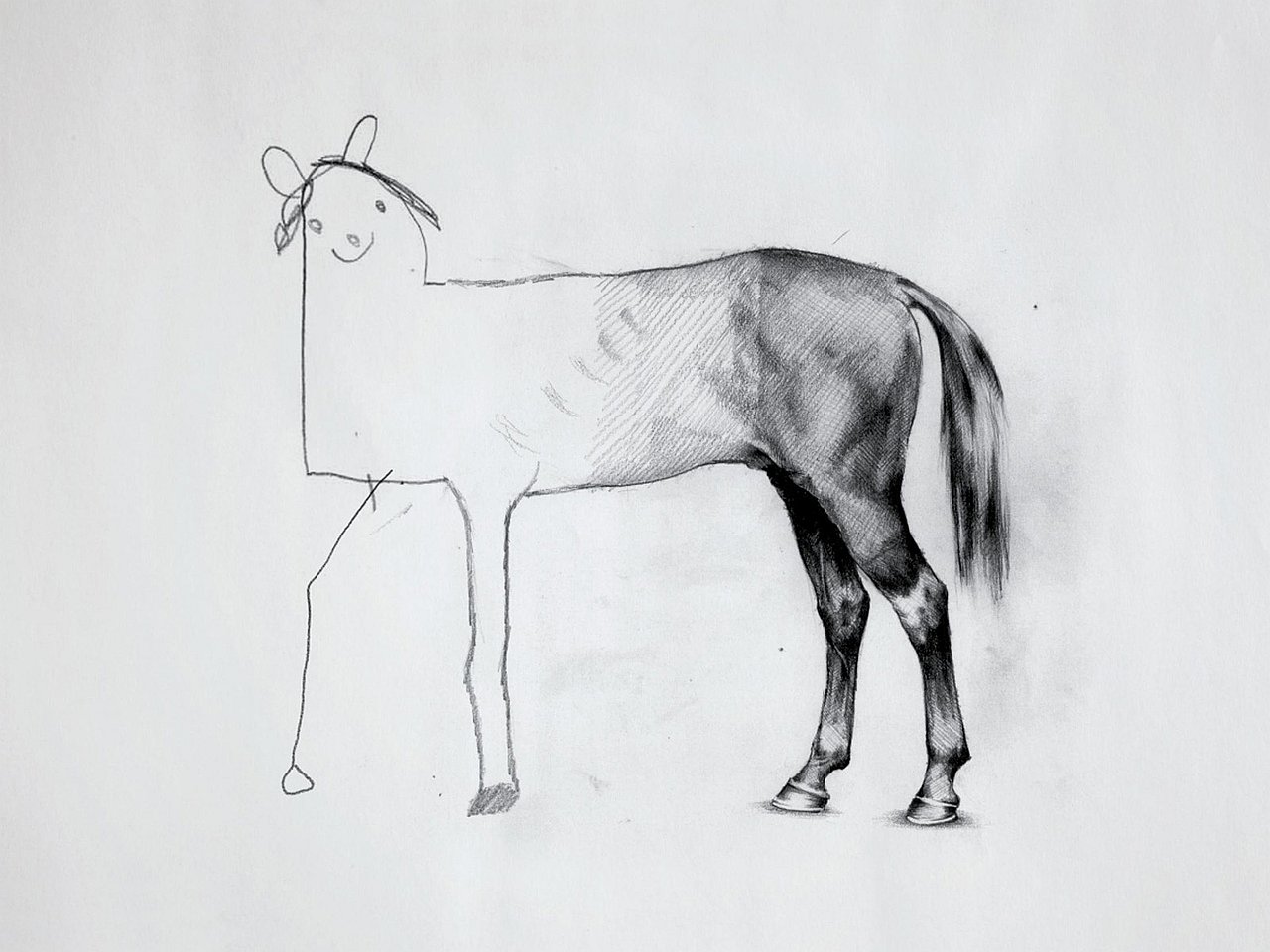
However, this numerical perspective represents just one facet of comprehending the world around us. We possess the ability to count and intuitively recognise the size of objects, but our perception also enables us to abstract away extraneous details and grasp the essential features such as the shape of objects, even in the presence of considerable noise. This phenomenon is prominently featured in various artistic movements, ranging from Cubism and Impressionism to abstract art. A tangible illustration of this is the widely recognised drawing “The Horse” by Ali Bati (see Figure ⁠1⁠), showcasing our capacity to perceive evolving forms and concepts amidst significant deformation and noise.

This artwork, which has become a popular meme, encapsulates the Platonic idea of shape. Despite significant deformation, we can still discern the concept of a horse in there. This human observation raises a crucial question: Are there mathematical notions that allow us to recognise a shape amidst substantial noise and distortion? The paper will cover state-of-the-art tools that address this query, delving into the basic formalism and algorithms. Additionally, various applications of the introduced methodology will be discussed.

2 Always visualise!

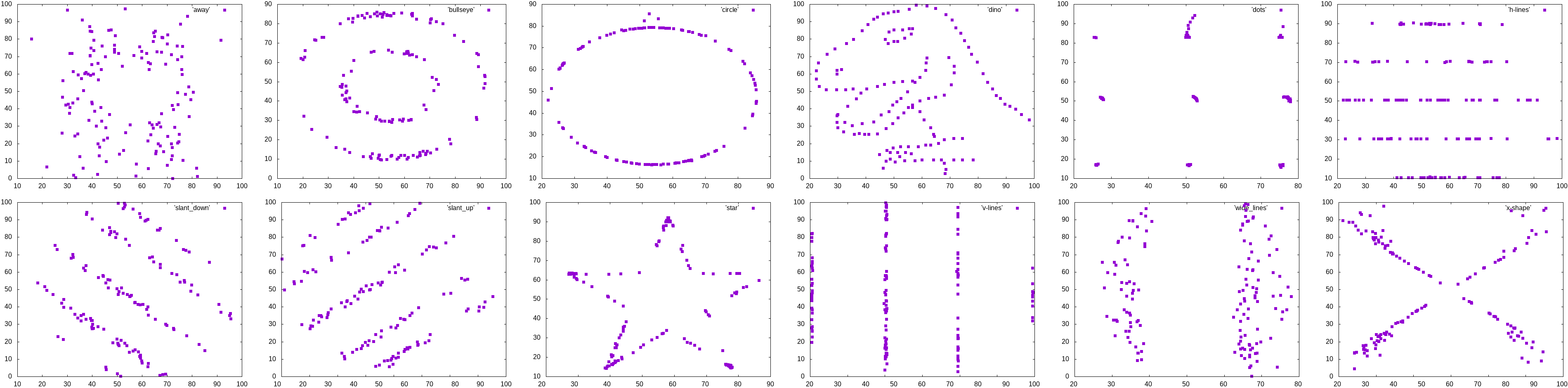
Before driving into topology, it is crucial to acknowledge that standard statistics already provide a range of basic analytical tools for discrete shapes. These include standard statistical moments, correlations between dimensions, and one- or two-sample statistical goodness-of-fit tests, which facilitate the comparison of various samples (a.k.a. point clouds). Although these methods have robust theoretical underpinnings and offer assurances of limit convergence, they encounter a notable limitation: they tend to condense the characteristics of often high-dimensional and complex shapes into a single numerical value, a statistical representation of the shape. From the era of Anscombe’s quartet [⁠1⁠] to the more recent Datasaurus dozen [⁠13⁠] illustrated in Figure ⁠2⁠, comes a persistent message urging for visualisation of data. This is because the sole reliance on statistical values may not be sufficient. The Datasaurus dozen, for instance, presents very different datasets that share nearly identical summary statistics.

Visualisation proves to be straightforward when handling two-dimensional samples. Yet, the vast majority of datasets are much higher dimensional, rendering direct visualisation a challenging task. To circumvent this issue, dimension reduction techniques are commonly employed, though they inevitably cause some loss of information. The topological methods discussed below offer a novel pathway for the visualisation and comprehension of data’s shape, effectively addressing the complexities associated with high-dimensional datasets.

3 Second star to the right and straight on till morning

Many classical topological characteristics of spaces are invariant under continuous deformations. This property has inspired a humorous adage among topologists, stating that they cannot distinguish between a coffee mug and a doughnut, as one can be continuously deformed into the other. This analogy, viewed positively, underscores the robustness of topology against substantial amounts of noise and deformation.

The study of invariants in topology dates back to 1758, when Euler discovered that for a convex polyhedron, the number of vertices (V), edges (E), and faces (F) are interconnected by the formula , regardless of the specific arrangement of vertices, edges, and faces. Euler’s insight precipitated at least two significant breakthroughs: firstly, it facilitated the representation of space using a finite set of information, thus effectively generalising the concept of an abstract graph, also introduced by Euler on occasion of solving the Königsberg bridge problem in 1736. Secondly, it provided one of the earliest topological characteristics of a space, which essentially states that every convex polygon has one connected component and encloses one cavity. Consequently, shapes with varying numbers of connected components or cavities exhibit distinct Euler characteristics.

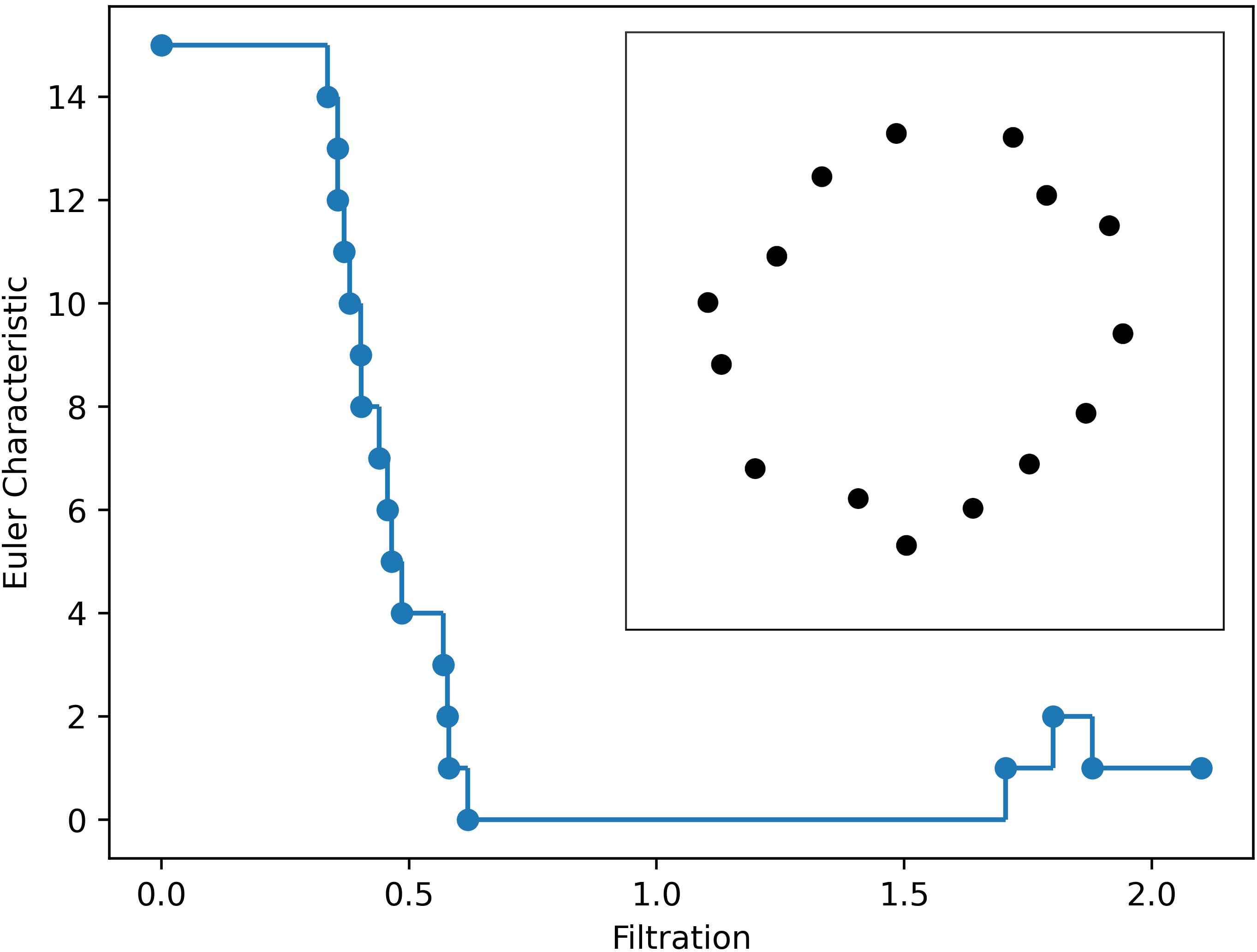
Traditionally, the Euler characteristic is defined for solids, while typical inputs in data analysis comprise a finite point sample . Formally, such a point sample represents a discrete collection of points, lacking any inherent geometrical structure. However, a metaphorical “squinting of our eyes” can reveal an underlying shape, particularly evident when examining the upper right panel of Figure ⁠4⁠.

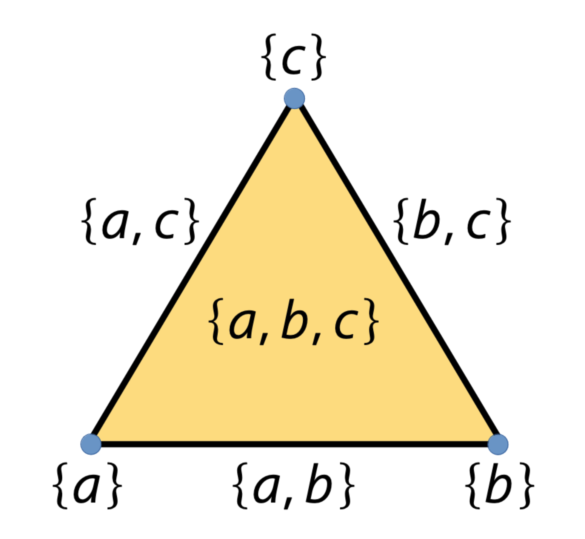
There are many ways in which the process of “squinting eyes” can be formalised. Let us start with the concept of an abstract simplicial complex [⁠9⁠] – a collection of sets that is closed under the operation of taking subsets. For instance, the collection satisfies this condition, as every subset of each set from  is also an element of . This particular simplicial complex represents a geometrically filled-in triangle. Elements of the complex are referred to as simplices. The dimension of a simplex , , is defined as one less than its cardinality. The alternating sum of the counts of simplices of successive dimensions, , gives the Euler characteristic of .

One of the earliest ways of constructing abstract simplicial complexes from point samples is attributed to Vietoris and Rips [⁠17⁠]. Given a finite sample  equipped with a metric  and a proximity parameter , this approach connects with an edge points in that are at most apart. Cliques in the resulting -neighbourhood graph correspond to simplices in the Vietoris–Rips complex. Since a sub-clique of a clique is itself a clique, we obtain a well-defined simplicial complex for every .

Although the Vietoris–Rips complex is relatively easy to define, it has a serious drawback. For sufficiently large , the size of the complex grows exponentially with respect to the cardinality of . To circumvent this problem, both topology and geometry need to be taken into account. First, take the union of balls of radius , centred at points from . Then restrict these balls to the Voronoi cells of their centres. The -fold nonempty intersections of those restricted balls correspond to simplices in the so-called alpha complex, see [⁠9⁠]. While more challenging to compute, alpha complexes offer the clear advantage of having sizes, under mild assumptions, proportional to the size of . Moreover, they can be effectively computed using CGAL and Gudhi, European software packages in computational geometry and topology, respectively.

Both of the presented constructions depend on the distance parameter , which serves as the resolution parameter. Since there is no canonical method for choosing a single value of , a whole range of radii, typically spanning from zero to infinity, is considered. Given two radii , the complex  obtained at radius  is a subset of the complex obtained at radius . Since both and  are complexes, we say that is a subcomplex of . In this scenario, each simplex is equipped with the value of  at which it appears for the first time, referred to as a filtration of the simplex.

This approach transforms the point sample into a multiscale combinatorial structure of a filtered simplicial complex that effectively summarises the data and formalises the “squinting eyes” process. For an example of filtered simplicial complex depending on a growing proximity parameter, please consult Figure ⁠3⁠.

4 Summaries of filtration: ECC

The classical concepts of Euler characteristics and filtration come together handily. By combining these methods and computing the Euler characteristic for each radius in a filtration we get a function called the Euler characteristic curve (ECC). It assigns to a radius the Euler characteristic of a complex and constitutes the most fundamental multiscale summary of the shape of the sample. Figure ⁠4⁠ exemplifies the ECC for the point sample at the upper right panel.

The Euler characteristic, advantageously positioned at the confluence of topology, differential geometry (as exemplified by the Gauss–Bonnet theorem), and vector calculus (illustrated by the Poincaré–Hopf theorem), emerges as a versatile and universal tool with a wide array of applications. Among its most notable uses is in cosmology, where it aids in understanding the geometry of both the current and early universe [⁠18⁠]. In this study, we shall explore another vital application, particularly pertinent to data analysis: the use of ECC in statistics, with a focus on goodness-of-fit tests.

In the classical statistical framework, we encounter two primary challenges: one-sample and two-sample goodness-of-fit problems. The one-sample test is employed to determine whether a set of points has been sampled from a known and explicitly defined probability density. On the other hand, the two-sample tests involve an additional finite sample, substituting for the probability density. The aim here is to determine whether the two provided samples are derived from the same probability density.

The availability of tools to address one-sample and two-sample goodness-of-fit problems is heavily influenced by the dimensionality of the data. For one-dimensional cases, there is a plethora of tools, including the Kolmogorov–Smirnov, Cramér–von Mises, Anderson–Darling, chi-squared, and Shapiro–Wilk tests, to name a few. These are supported by multiple efficient computational tools implemented in various programming languages. In two-dimensional cases, theoretical results for the Kolmogorov–Smirnov and Cramér–von Mises tests are available, along with some implementations in Python and R. However, for higher-dimensional data, while theoretical results for the Kolmogorov–Smirnov test exists, only a handful of implementations are available.

Standard tests primarily rely on the cumulative distribution function (CDF) of a real-valued random variable  that, at a given point , determines the probability of  being less than or equal to . Generalising this concept to higher-dimensional data poses significant challenges with current implementations, as it necessitates considering all permutations of the data axes.

However, topological characteristics of a sample, such as the Euler characteristic curve, are invariant under multiple data transformations, including permutations of the axes and affine transformations. While providing slightly weaker invariants, they do not encounter the same problems as traditional methods including CDF. In our recent work [⁠7⁠], the ECC of a sample is utilised as a surrogate for the cumulative distribution function, yielding an efficient statistical test that surpasses the state of the art. This new family of tests, referred to as TopoTests, has proven to outperform existing methods even in low-dimensional and small data samples scenarios.

To illustrate it, consider the matrices in Figure ⁠5⁠. The value at position in each matrix indicates the power of the test, defined as the probability that the test successfully recognises that a sample, in this case of size 100, taken from the distribution in the -th row, does not originate from the distribution in the -th column. When , the value on the diagonal represents the confidence level for which the test was designed. It is therefore supposed to reject the true hypothesis in of cases.

Figure ⁠5⁠ showcases the performance comparison between the Kolmogorov–Smirnov test (left) and TopoTests (right) for a three-dimensional sample. In the colouring scale used in the figure, a better test can be recognised as one with more yellow entries in the matrix. In this instance, TopoTests consistently outperform the standard Kolmogorov–Smirnov test, illustrating the potential applicability of topological tools in statistical analysis. As described in [⁠7⁠], TopoTests can be easily accessed and utilised through a public domain implementation.

It is noteworthy that this approach comes with asymptotic theoretical guarantees. It is also important to be mindful that in some rare instances, the Euler characteristic curves of different distributions may be quite similar, leading to less effective performance of the test. These occasional limitations are a trade-off for the additional advantages offered by the proposed TopoTests. Please consult [⁠7⁠] for further details.

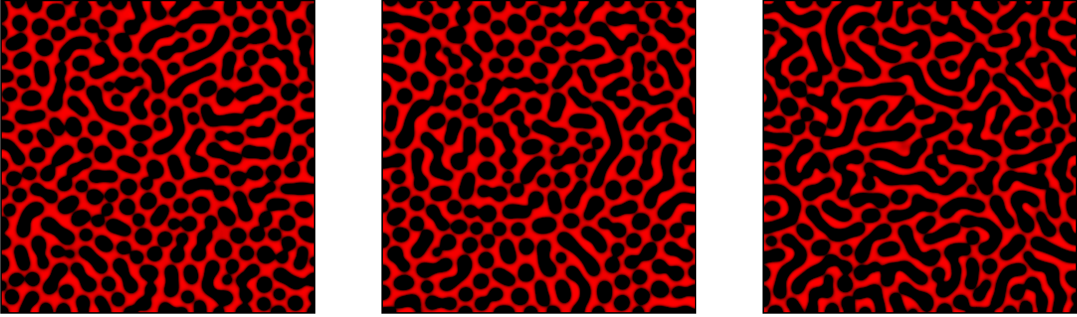
Integrating topology with statistics offers an additional significant advantage: it extends the application of statistical goodness-of-fit tests to a broader range of inputs, specifically those for which an ECC can be calculated. For instance, inputs in the form of a scalar-valued function on a bounded domain, such as an image (referenced in Figure ⁠6⁠), can be processed in this framework. In this figure we see a visualisation of three solutions of the Cahn–Hilliard–Cook equation,

where for every in the domain of (in this case, the unit square). The constant is the total mass, see [⁠8⁠] for details. The three solutions illustrated in Figure ⁠6⁠ represent for a fixed and the initial condition , and , respectively. It turns out that the information about the initial condition  as well as the time  at which the solution is obtained can be recovered from the topology of the patterns in Figure ⁠6⁠. In this case, the first two images, corresponding to , depict “drop-like” formations, while the third image, associated with , exhibits a snake-like behaviour. For a preliminary study on this, refer to [⁠8⁠]. This example illustrates that the topological approach enables us to broaden the scope of data types that can be analysed using standard statistical methods

5 Summaries of filtration: persistence

While the ECC is nice and simple, TDA offers a more advanced multiscale invariant of data: persistent homology. From persistent homology, also referred to as persistence, one can easily obtain the ECC, but not vice versa. Persistent homology is a multiscale version of the homology theory briefly outlined below.

Suppose we have an abstract simplicial complex obtained from a sample for fixed radius using either the Vietoris–Rips, or the alpha complex construction. Homology recovers information about connectivity of in different dimensions. At dimension 0, homology recovers connected components of . Focusing on the filtration presented in Figure ⁠3⁠, in step (1) there are five connected components (corresponding to points of ), three at the level (2), two at level (3), and a single connected component since after. Homological features of dimensions are represented by classes of one-dimensional cycles that do not bound any collection (or formally, a chain) composed of two-dimensional simplices. Such a cycle can be observed at the step (4) of the filtration. We can intuitively think about them as bounding “one-dimensional holes” in the complex. The story continues for higher dimensions, where homology theory detects features, informally bounding higher-dimensional holes in the considered complex.

Persistent homology enables tracking of the homological features, such as connected components and holes of dimension one or higher, as the filtration of the complex evolves. During this process, homology classes are created and then some of them cease to exist. Consider for example the one-dimensional cycle from step (4) of Figure ⁠3⁠ – it appears (is born) at step (4) and ceases to exist (dies) at step (5), becoming the boundary of two two-dimensional simplices added in step (5). The persistence interval, presented in red in Figure ⁠3⁠, spans the filtration values in which the one-dimensional topological feature exists. A similar narrative applies to homological features in dimension . For instance, consider the three leftmost points of  in step (1) of the filtration. They become connected at step (2), forming a single component. Consequently, two of them cease to exist, giving rise to two persistence intervals in zero-dimensional persistent homology. The collection of persistence intervals for the filtration at the top of Figure ⁠3⁠ is given at the bottom of the figure. Persistence intervals of various filtrations can be compared using for instance distances developed to solve optimal transport problems.

In this short exposition we have barely scratched the surface of persistent homology. For a comprehensive introduction, please consider [⁠9⁠].

6 Questions you did not know you had

“Visualisation gives you answers to questions you didn’t know you had” – this famous quote by Ben Shneiderman encapsulates a fundamental desire in various scientific fields: to discern patterns, formulate hypotheses about underlying principles, and subsequently verify them. Topological data analysis offers tools to visualise high-dimensional data through the so-called mapper algorithm. Introduced in 2007 by Gunnar Carlsson and coauthors [⁠16⁠], the mapper algorithm represents a given high-dimensional sample as an abstract graph, termed a mapper graph. Since its inception, the mapper algorithm has had a significant academic and industrial impact, boasting hundreds of successful applications and numerous industrial implementations, including extensive work by Symphony AyasdiAI.

A general method to derive a mapper graph from a point sample  is straightforward: one needs to construct an overlapping cover of , namely, a collection of subsets such that and . Subsequently, a graph called the one-dimensional nerve of the cover is built. This abstract graph’s vertices correspond to elements of the cover, and its edges represent the nonempty intersections of these elements, as illustrated in Figure ⁠7⁠. The mapper graph models a space  upon which a function can be visualised. This can be achieved, for example, by calculating the average value of  for each . The value at the vertex of the graph corresponding to  can then be visualised using an appropriate colour scale.

There are two main methods to construct such an overlapping cover. The first one, proposed in [⁠16⁠], originates from the Reeb graph construction. Initially,  is mapped into using a so-called lens function . The interval is then covered by a series of overlapping elements , with each consecutive pair having a nonempty overlap. For each , a clustering algorithm is then applied, and the obtained clusters are used as cover elements. As and overlap, this results in an overlapping cover of .

The second construction, proposed in [⁠5⁠], leading to a ball mapper graph, involves a fixed and a metric  on . An -net is built on , defined as a subset such that for every , there exists with . Consequently, and the family of balls for forms an overlapping cover of .

Topological visualisation tools, such as mapper graphs, have a plethora of applications across various fields. We have selected two examples, one from social sciences and the other from material design.

In the realm of social sciences, we explore the phenomenon of Brexit – the process leading to the outcome of the UK’s 2015 referendum, where a majority of voters decided for the UK to leave the EU. Our analysis, presented in [⁠15⁠], is based on the 2012 census data and superimposed it with the Brexit referendum results at the constituency level.

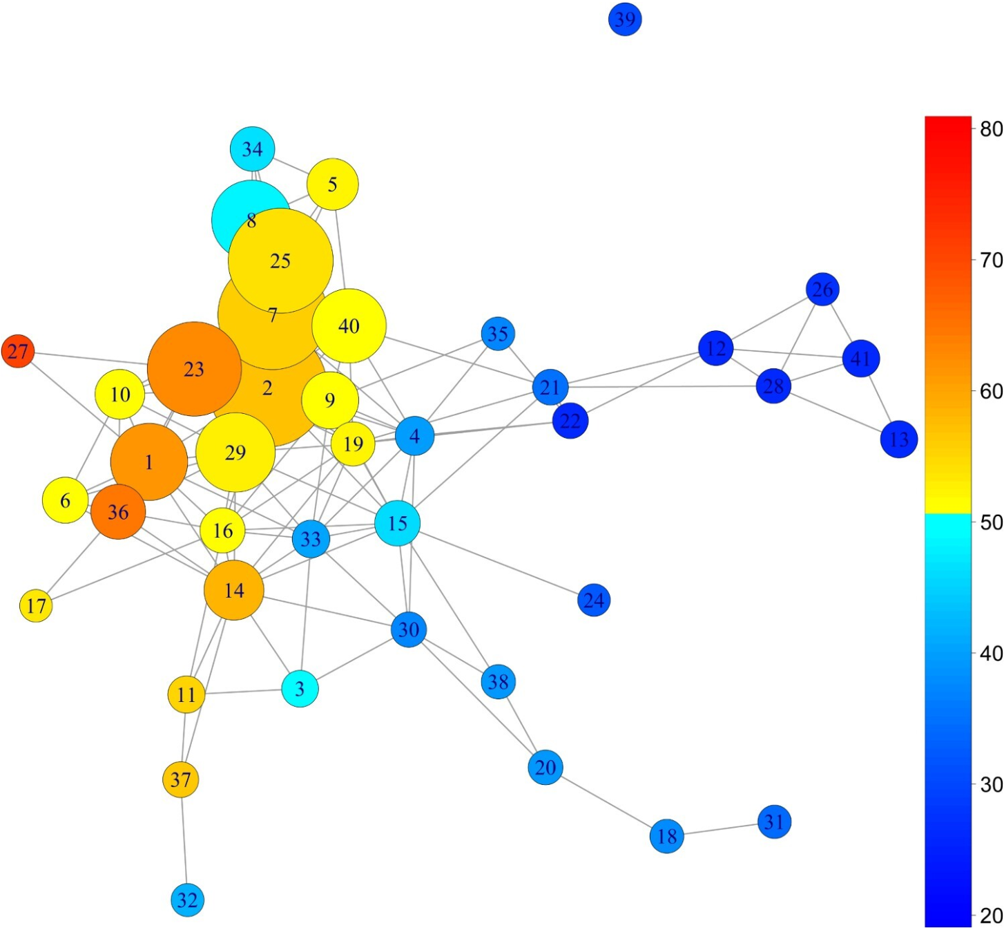
The ball mapper graph, thoroughly discussed in [⁠15⁠], is depicted in Figure ⁠8⁠. Despite the substantial aggregation of information, several sociological observations emerge. The most notable among them is the relative homogeneity (at a sociological level) of the constituencies supporting Brexit (marked with yellow and orange), contrasted with the vast heterogeneity of those favouring the UK’s continued membership in the EU (marked with blue). This observation, along with multiple other conclusions and hypotheses, is elaborated upon in [⁠15⁠].

Our second example, elaborated in detail in [⁠12⁠], pertains to descriptors of three-dimensional porous structures of hypothetical zeolites. Zeolites are chemically-simple nanoporous structures derived from SiO tetrahedra, assembled into hundreds of thousands of different crystal structures. Although primarily used in detergents to soften water, zeolites have the potential for applications in gas capture and storage (such as methane and carbon dioxide), noble gas separation, and other areas. Given their chemical simplicity, the defining factor for the properties of a given material is the shape of its pores. In the study [⁠12⁠], this shape is characterised using the persistent homology of points sampled from the pores’ surfaces. The persistence intervals of successive dimensions obtained for a given material serve as the material’s features. They allow inducing a distance function between different materials as the distance between the persistence diagrams obtained from them, see [⁠9⁠].

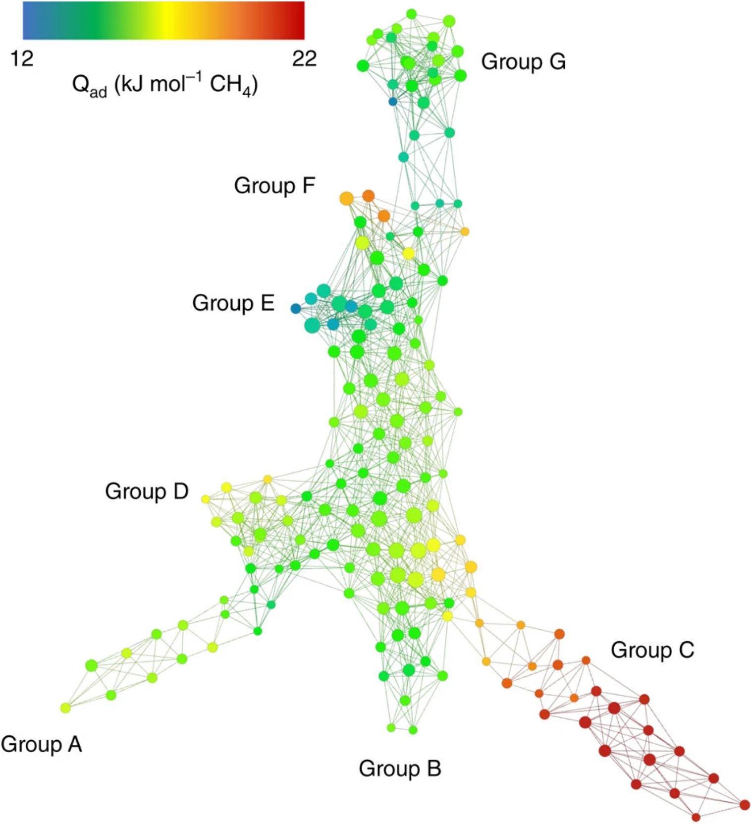
The presented approach gives us a discrete metric space representing the considered database of hypothetical zeolites. A mapper graph, representing the shape of this space, is illustrated in Figure ⁠9⁠. The graph uses a colouring function based on the heat of absorption, which determines the temperature at which a given material can absorb the maximum amount of gas, in this case, methane. We observe that this property appears to be “continuously dependent” on the material’s shape. Furthermore, different regions of this space, denoted by distinct groups in the graph, correspond to various humanly-interpretable geometries of pores. This research highlights the synergy between statistics and machine learning-friendly topological descriptors (such as persistent homology), and topological visualisation. This combination provides a comprehensive overview of the shape of the space of hypothetical zeolites. The colouring function enables the identification of regions in the space containing materials with the desired values of properties of interest.

7 Multiple filtrations at once?

The filtrations considered thus far have focused on a single aspect of the data – either the mutual distances between points, or the greyscale intensity values of an image’s pixels. However, scenarios exist where examining multiple characteristics concurrently is necessary. For instance, in the context of images, one might consider multiple channels, such as RGB. With point samples,

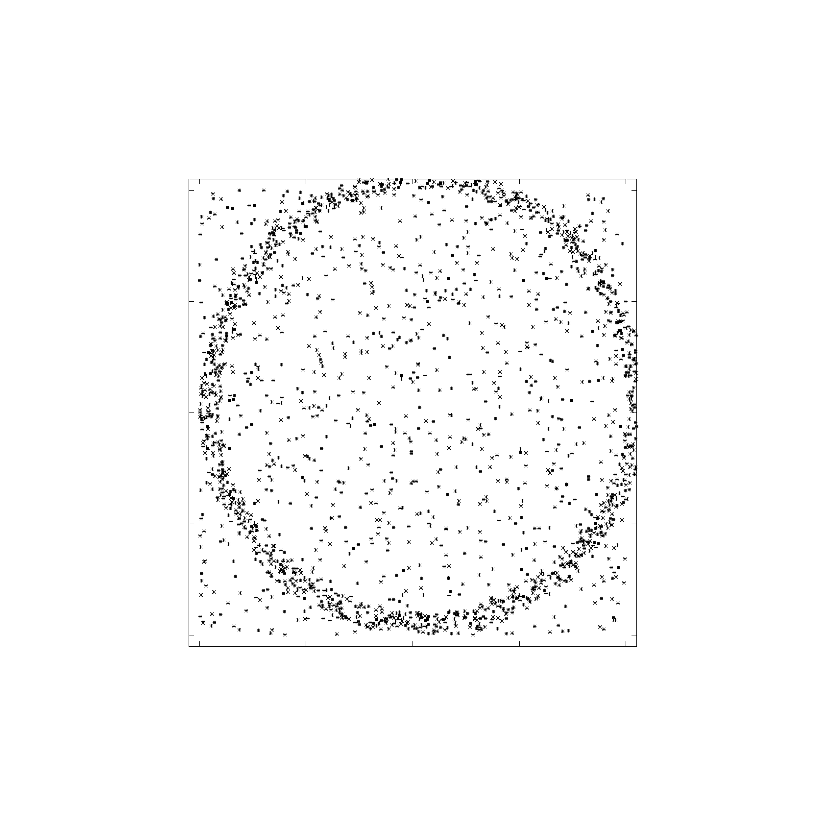
envision a set of points sampled from a circle but contaminated with a lower density of uniform noise inside the circle. While our brain is adept at discerning the shape of a circle despite the noise, a clear persistent interval might not be obtained with a filtration based solely on distances. The inclusion of additional filtration parameters, like local density, becomes necessary. However, effective generalisations of persistent homology to multiple filtration parameters have proven to be a serious challenge. This is due to problems rooted in representation theory, which pose an obstruction against the existence of a counterpart to persistence intervals, see [⁠3⁠]. This is the case despite the considerable collective efforts of the TDA community.

Addressing the challenges in generalising persistent homology, we return to the foundational concept of the Euler characteristic. Specifically, its parametric version, the Euler characteristic curve, at a given radius , is essentially an alternating sum of the number of simplices of successive dimensions. Once a simplex enters the filtration, it remains therein, contributing to the alternating sum and hence the ECC. Therefore, the contribution of simplex to the ECC is an indicator function; it equals 0 for all arguments below the simplex’s filtration value and 1 thereafter. The ECC we have considered so far is the alternating sum of such indicator functions.

This simple observation paves the way to generalise the ECC for the case of multidimensional filtrations. It is conceivable that a simplex  appears at one or several non-comparable points in an -dimensional filtration. In such cases, simplex  will contribute a value of 1 at every point that is coordinate-wise greater or equal to any of , and 0 at all other points. Through this method, we obtain a stable invariant of an -dimensional filtration, referred to as the Euler characteristic profile, see [⁠6⁠] for further discussion and properties.

Let us consider a simple example of such a scenario: a problem of analysing prostate cancer features on hematoxylin and eosin (H&E) stained slide images. Our results are based on publicly available 5182 images, each of resolution, obtained from the Open Science Framework [⁠11⁠], as analysed in [⁠6⁠]. These images represent various regions of interest (ROIs) from prostate cancer H&E slices, collected from 39 patients. The unique aspect of each image is its annotation with a Gleason score, 3, 4, or 5, reflecting the architectural patterns of the cancer cells. A higher Gleason score is indicative of increased cancer aggressiveness.

Given such an annotated dataset, a natural question arises: can a Gleason scale assigned by a histopathologist be deduced from the shape of the structures visible in Figure ⁠10⁠ using appropriate regression techniques applied to topological characteristics of images? For this purpose, methods of persistent homology and Euler characteristics have been employed, achieving an accuracy of approximately 76%. The utilisation of Euler characteristic profiles utilising both H&E channels further enhanced the accuracy to 82%. In both instances, random forest regression methods were applied. This example illustrates that considering multiple filtrations simultaneously can lead to significant improvements in performance of the data analysis tools.

8 Summary

“Data has shape, shape has meaning, and meaning brings value” – this foundational quote by Gunnar Carlsson encapsulates the essence of topological data analysis: to seek out rich and robust features that summarise the geometric and topological structure of complex and high-dimensional datasets. Now, after nearly 20 years of development, the field boasts many success stories and offers a wealth of tools to the community. In informal conversations, I often refer to the tools we provide as “statistics on steroids” – they go beyond relying on single numbers and embrace much more complex features, while retaining (almost) all the properties of standard statistics. In addition, they are directly applicable to standard algorithms in statistics [⁠2⁠], machine learning [⁠14⁠] and AI [⁠4⁠].

Among other initiatives, my Dioscuri Centre in Topological Data Analysis is contributing new tools to the field and the whole scientific community. We work closely with domain experts in mathematics, medicine, economics, finance, physics, biology, and more, aiming to integrate our new tools into the daily practice of applied mathematicians and researchers utilising mathematics in their fields. If you are interested in our research, please visit our web page. All the theoretical tools described in this paper are implemented and freely available at our GitHub page.⁠¹⁠

Acknowledgements. The author would like to thank Krzysztof Burnecki for the kind invitation to write this article. The author acknowledges the support by the Dioscuri Programme initiated by the Max Planck Society, jointly managed with the National Science Centre (Poland), and mutually funded by the Polish Ministry of Science and Higher Education and the German Federal Ministry of Education and Research, as well as M-ERA.NET PORMETALOMICS and MRC-GAP projects. I am grateful to all my students, postdocs and collaborators for the joint research discussed in this paper. I received excellent feedback in the preparation of this manuscript and would like to extend my thanks to (in alphabetical order): Grzegorz Graff, Davide Gurnari, Niklas Hellmer, Simon Rudkin, Radmila Sazdanovic, Justyna Signerska-Rynkowska and Rafał Topolnicki.

Paweł Dłotko is the leader of the Dioscuri Centre in Topological Data Analysis at the Mathematical Institute of the Polish Academy of Sciences in Warsaw, Poland. He is a 2012 graduate of Jagiellonian University in Krakow, Poland, he has diverse experience from positions at Swansea University (UK), Inria Saclay (France), University of Pennsylvania (USA), and more. His expertise lies in applied and computational topology, focusing on mathematically rigorous data descriptors. Paweł is a prolific applied mathematician and computer scientist, known for developing numerous algorithms and computational libraries in topological data analysis.⁠²⁠pdlotko@impan.pl

1. ¹

   https://github.com/dioscuri-tda/

2. ²

   Please see https://dioscuri-tda.org/members/pawel and https://scholar.google.com/citations?user=-_znDLoAAAAJ for further details.

References

1. F. J. Anscombe, Graphs in statistical analysis. Amer. Statist. 27, 17–21 (1973)
2. P. Bubenik and P. Dłotko, A persistence landscapes toolbox for topological statistics. J. Symbolic Comput. 78, 91–114 (2017)
3. G. Carlsson and A. Zomorodian, The theory of multidimensional persistence. In Computational geometry (SCG’07), pp. 184–193, ACM, New York (2007)
4. M. Carrière, F. Chazal, Y. Ike, T. Lacombe, M. Royer and Y. Umeda, PersLay: A neural network layer for persistence diagrams andnew graph topological signatures. In: Proceedings of the Twenty Third International Conference on Artificial Intelligence andStatistics, Proc. Mach. Learn. Res. (PMLR) 108, pp. 2786–2796,PMLR (2020)
5. P. Dłotko, Ball mapper: a shape summary for topological data analysis. arXiv:1901.07410v1 (2019)
6. P. Dłotko and D. Gurnari, Euler characteristic curves and profiles: a stable shape invariant for big data problems. GigaScience 12, article no. giad094 (2023)
7. P. Dłotko, N. Hellmer, Ł. Stettner and R. Topolnicki, Topology-driven goodness-of-fit tests in arbitrary dimensions. Stat. Comput. 34, article no. 34 (2024)
8. P. Dłotko and T. Wanner, Topological microstructure analysis using persistence landscapes. Phys. D 334, 60–81 (2016)
9. H. Edelsbrunner and J. L. Harer, Computational topology. American Mathematical Society, Providence, RI (2010)
10. P. Lawson, A. B. Sholl, J. Q. Brown, B. T. Fasy and C. Wenk, Persistent homology for the quantitative evaluation of architectural features in prostate cancer histology. Sci. Rep. 9, article no. 1139 (2019)
11. P. Lawson, C. Wenk, B. T. Fasy and J. Brown, Persistent homology for the quantitative evaluation of architectural features in prostate cancer histology. OSF (2020) DOI 10.17605/OSF.IO/K96QW
12. Y. Lee, S. D. Barthel, P. Dłotko, S. M. Moosavi, K. Hess and B. Smit, Quantifying similarity of pore-geometry in nanoporous materials. Nat. Commun. 8, article no. 15396 (2017)
13. J. Matejka and G. Fitzmaurice, Same stats, different graphs: Generating datasets with varied appearance and identical statistics through simulated annealing. In Proceedings of the 2017 CHI Conference on Human Factors in Computing Systems, pp. 1290–1294, Association for Computing Machinery, New York (2017)
14. J. Reininghaus, S. Huber, U. Bauer and R. Kwitt, A stable multi-scale kernel for topological machine learning. In 2015 IEEE Conference on Computer Vision and Pattern Recognition (CVPR), pp. 4741–4748, IEEE, Boston, MA (2015)
15. S. Rudkin, L. Barros, P. Dłotko and W. Qiu, An economic topology of the Brexit vote. Reg. Stud. 58, 601–618 (2024)
16. G. Singh, F. Mémoli and G. Carlsson, Topological methods for the analysis of high dimensional data sets and 3D object recognition. In Eurographics Symposium on Point-Based Graphics, pp. 91–100, The Eurographics Association, Goslar, Germany (2007)
17. L. Vietoris, Über den höheren Zusammenhang kompakter Räume und eine Klasse von zusammenhangstreuen Abbildungen. Math. Ann. 97, 454–472 (1927)
18. R. van de Weygaert, G. Vegter, H. Edelsbrunner, B. J. T. Jones, P. Pranav, C. Park, W. A. Hellwing, B. Eldering, N. Kruithof, E. G. P. Bos, J. Hidding, J. Feldbrugge, E. ten Have, M. van Engelen, M. Caroli and M. Teillaud, Alpha, Betti and the megaparsec universe: on the topology of the cosmic web. In Transactions on computational science XIV, Lecture Notes in Comput. Sci. 6970, pp. 60–101, Springer, Heidelberg (2011)