
For electricity grid operators, the planning of grid operations depends on having accurate models for forecasting wind power production on a number of different time resolutions. Together, these time resolutions create what has become known as a temporal hierarchy. Previous studies have considered methods of reconciling forecast hierarchies inspired by least squares methodologies that produce coherent and more accurate forecasts. In this study, we highlight some challenges in the established approach when applied to wind power production, and consider methods which more appropriately take into account the full conditional probability densities. We suggest methods using maximum likelihood techniques to estimate the prediction variance ahead of time. Using base forecasts from a commercial forecast provider together with simpler forecasting models, we test the modified approach against the established reconciliation approach on data from Danish wind farms. The results show significant improvements in accuracy when compared to both the state-of-the-art commercial forecasts and the simpler models.
Introduction
As part of the ongoing green transition, the share of renewable energy being incorporated into the electricity grid is increasing. With this comes the challenge of renewable energy sources, such as wind power, being stochastic in nature, i.e., power production depends on, e.g., the wind speed. Thus, in order to plan and control the electricity grid, transmission system operators (TSOs) require reliable and accurate forecasts of power production. With targets such as the European Union having 70% of power production stemming from renewable energy sources by 2050,1IRENA, Global energy transformation: A roadmap to 2050; https://www.irena.org/publications/2019/Apr/Global-energy-transformation-A-roadmap-to-2050-2019Edition. this challenge is only becoming greater. Hence, the importance of accurate and reliable wind power forecasts is more crucial now than ever before.
The main goal in this respect is thus to reduce the uncertainty of the forecasted power production as much as possible. One of the more recent developments within forecasting, which has been shown to reduce the forecast uncertainty, is the method of hierarchical forecast reconciliation. The method in its current form was suggested by [7 R. J. Hyndman, R. A. Ahmed, G. Athanasopoulos and H. L. Shang, Optimal combination forecasts for hierarchical time series. Comput. Statist. Data Anal. 55, 2579–2589 (2011) ], with further developments by [8 R. J. Hyndman, A. J. Lee and E. Wang, Fast computation of reconciled forecasts for hierarchical and grouped time series. Comput. Statist. Data Anal. 97, 16–32 (2016) , 17 S. L. Wickramasuriya, G. Athanasopoulos and R. J. Hyndman, Optimal forecast reconciliation for hierarchical and grouped time series through trace minimization. J. Am. Stat. Assoc. 114, 804–819 (2019) , 14 P. Nystrup, E. Lindström, P. Pinson and H. Madsen, Temporal hierarchies with autocorrelation for load forecasting. Eur. J. Oper. Res. 280, 876–888 (2020) ]. Hierarchical forecast reconciliation utilizes the hierarchical structures that are often naturally present in data by ensuring that forecasts on different resolutions are coherent. Coherency refers to the fact that the layers should add up throughout the hierarchy in a natural way. An example of this comes from the study on Australian domestic tourism by [1 G. Athanasopoulos, R. A. Ahmed and R. J. Hyndman, Hierarchical forecasts for Australian domestic tourism. Int. J. Forecast. 25, 146–166 (2009) ], where forecasts are produced at the national scale, state scale, zone scale, and regional scale. These forecasts form a hierarchy, where one would expect that all the regional forecasts within a zone add up to the zone forecast, all the zone forecasts within a state add up to the state forecast, etc. When forecasts add up in this manner, the forecasts are said to be coherent. However, when the forecasts on each layer are produced independently of each other this will not be the case. The purpose of hierarchical forecast reconciliation is thus to produce a set of reconciled forecasts that have the coherency property based on a set of incoherent base forecasts.
Hierarchies can be either spatial, as was the case for the example on Australian domestic tourism, temporal, as has been explored by [2 G. Athanasopoulos, R. J. Hyndman, N. Kourentzes and F. Petropoulos, Forecasting with temporal hierarchies. Eur. J. Oper. Res. 262, 60–74 (2017) ] and [14 P. Nystrup, E. Lindström, P. Pinson and H. Madsen, Temporal hierarchies with autocorrelation for load forecasting. Eur. J. Oper. Res. 280, 876–888 (2020) ], or spatio-temporal, e.g., [9 N. Kourentzes and G. Athanasopoulos, Cross-temporal coherent forecasts for Australian tourism. Ann. Tourism Res. 75, 393–409 (2019) ]. In a spatial hierarchy one might examine regional forecasts, see, e.g., [7 R. J. Hyndman, R. A. Ahmed, G. Athanasopoulos and H. L. Shang, Optimal combination forecasts for hierarchical time series. Comput. Statist. Data Anal. 55, 2579–2589 (2011) ]. In a temporal hierarchy, which will be the case for this study, the forecasts should add up based on the timescale such that, e.g., the three monthly forecasts within a quarter add up to quarterly forecasts, and the four quarterly forecasts add up to yearly forecasts.
Forecast reconciliation of temporal hierarchies has shown great promise in reducing the uncertainty of the base forecasts and producing more accurate forecasts at all layers [14 P. Nystrup, E. Lindström, P. Pinson and H. Madsen, Temporal hierarchies with autocorrelation for load forecasting. Eur. J. Oper. Res. 280, 876–888 (2020) ]. However, the majority of studies on temporal hierarchies only show such improvements using simple models to produce the base forecasts, such as the ARIMA and exponential smoothing models by [2 G. Athanasopoulos, R. J. Hyndman, N. Kourentzes and F. Petropoulos, Forecasting with temporal hierarchies. Eur. J. Oper. Res. 262, 60–74 (2017) ]. These models also often require constant data availability, which under real-time operational conditions cannot always be guaranteed. The established reconciliation approach also assumes that the covariance structure between the forecasts is constant in time, which for many applications may not be the case. For wind power production it is well-known that the forecast uncertainty is highly dependent on, e.g., the wind speed [13 H. A. Nielsen, H. Madsen and T. S. Nielsen, Using quantile regression to extend an existing wind power forecasting system with probabilistic forecasts. Wind Energ. 9, 95–108 (2006) ]. Furthermore, wind power production is naturally bounded between zero and the installed capacity, which poses a challenge when reconciling, since the established method of reconciling assumes unbounded data. These challenges call for more refined methods to generate reconciled forecasts.
In the literature, forecast reconciliation has been applied previously to cases of both wind power forecasting and solar power forecasting, which both face similar issues. The paper [16 M. L. Sørensen, P. Nystrup, M. B. Bjerregård, J. K. Møller, P. Bacher and H. Madsen, Recent developments in multivariate wind and solar power forecasting. WIREs Energy Environ. 12, article no. e465 (2023) ] provides a brief overview of the literature on this. In [6 M. E. Hansen, P. Nystrup, J. K. Møller and H. Madsen, Reconciliation of wind power forecasts in spatial hierarchies. Wind Energ. 26, 615–632 (2023) ] the authors test some of the current methods for forecast reconciliation in a spatial hierarchy with a similar dataset to our case study and are able to achieve significant improvements in accuracy. They do not, however, account for the issue of the non-constant variance structure. The need for varying and mean-dependent variance when reconciling forecasts has also been highlighted by [3 H. G. Bergsteinsson, J. K. Møller, P. Nystrup, Ó. P. Pálsson, D. Guericke and H. Madsen, Heat load forecasting using adaptive temporal hierarchies. Appl. Energ. 292, article no. 116872 (2021) ] for the case of heat load forecasts, although the approach therein mostly addresses slower seasonal variations. Additionally, [18 S. L. Wickramasuriya, B. A. Turlach and R. J. Hyndman, Optimal non-negative forecast reconciliation. Stat. Comput. 30, 1167–1182 (2020) ] demonstrates a method of changing the forecast reconciliation methodology to account for non-negativity.
The purpose of the present study is thus:
To use real measurements and weather forecasts to examine whether improvements to commercial state-of-the-art wind power production forecasts can be achieved through forecast reconciliation.
To propose adjustments to the established reconciliation approach (MinT-Shrink by [17 S. L. Wickramasuriya, G. Athanasopoulos and R. J. Hyndman, Optimal forecast reconciliation for hierarchical and grouped time series through trace minimization. J. Am. Stat. Assoc. 114, 804–819 (2019) ]), which addresses the level and time-dependent covariance structure in the wind power framework.
This study is structured such that Section 1 introduces the concept of forecast reconciliation. Section 2 presents the wind power production data used in the study. Section 3 then examines how base forecasts are produced, and introduces the proposed adjustments to the reconciliation process. Section 5 shows the results, and lastly Section 6 concludes on the findings and gives some further perspectives.
1 Forecast reconciliation
For the temporal hierarchy in this study, prediction horizons up to 24 hours will be examined. So, to introduce the concepts of reconciling forecasts based on temporal hierarchies, a simple example hierarchy is constructed within the 24-hour prediction frame with 6-hour, 12-hour and 24-hour forecast resolutions. This example could, e.g., cover the total wind power production in the stated intervals. The hierarchical structure of this example is illustrated in Figure 1.
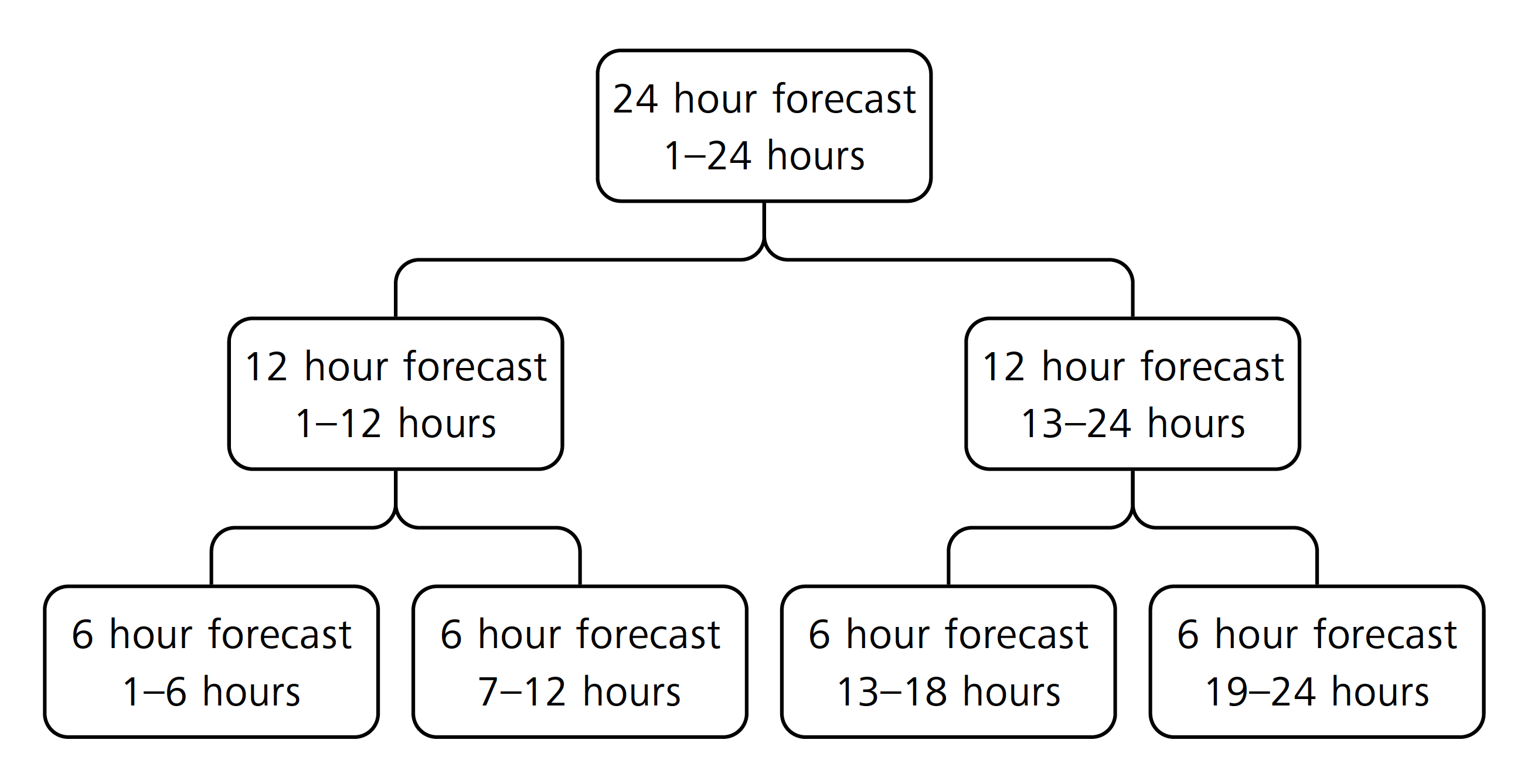
As illustrated by the figure, for such a hierarchy of forecasts to be coherent, the bottom-level 6-hour forecasts should add up pairwise to the second level 12-hour forecast, and the two 12-hour forecasts should add up to the highest level daily forecast. This summation property of the hierarchy is described by a summation matrix , where is the number of individual base forecasts (in this case 7) and is the number of forecasts on the lowest resolution (in this case 4). For the hierarchy in Figure 1, the summation matrix is given by:
The rows of the summation matrix define how the four bottom-level forecasts add up to each level of the hierarchy, so, e.g., the top-level forecast should be equal to the sum of all the four bottom-level forecasts. This also implies that the base forecasts () are ordered from top to bottom, i.e.
For clarity, the notation in this study uses superscripts for naming or other distinctions and subscripts for indices, so, e.g., is the forecast on the 6-hour resolution 13 to 18 hours ahead.
With the summation matrix and the base forecasts as defined above, the most commonly used method of forecast reconciliation, the MinT-Shrink [17 S. L. Wickramasuriya, G. Athanasopoulos and R. J. Hyndman, Optimal forecast reconciliation for hierarchical and grouped time series through trace minimization. J. Am. Stat. Assoc. 114, 804–819 (2019) ], can be introduced.
The method is based on a generalized least squares approach, which minimizes the coherency errors, i.e., the difference between the reconciled forecast () and the base forecast (). This implies solving the following optimization problem
where is the covariance matrix of the coherency errors , and . If is assumed to be known, the problem has a closed form solution, given by
In [17 S. L. Wickramasuriya, G. Athanasopoulos and R. J. Hyndman, Optimal forecast reconciliation for hierarchical and grouped time series through trace minimization. J. Am. Stat. Assoc. 114, 804–819 (2019) ] the authors showed that is not identifiable; instead, they propose the trace minimization approach (MinT), which uses the covariance matrix of the base forecast errors, i.e.,
where with being the observations arranged similarly to the base forecasts in equation (1). This approach has shown great promise in increasing forecast accuracy across all levels of the hierarchy. MinT-Shrink, also proposed by [17 S. L. Wickramasuriya, G. Athanasopoulos and R. J. Hyndman, Optimal forecast reconciliation for hierarchical and grouped time series through trace minimization. J. Am. Stat. Assoc. 114, 804–819 (2019) ], and extended to temporal hierarchies by [14 P. Nystrup, E. Lindström, P. Pinson and H. Madsen, Temporal hierarchies with autocorrelation for load forecasting. Eur. J. Oper. Res. 280, 876–888 (2020) ], is an extension of the MinT approach which applies a shrinkage estimator to the correlation.
The method estimates the covariance from the correlation matrix of the base forecast errors using the shrinkage parameter :
where is the so-called hierarchical variance, which is a diagonal matrix consisting of the empirical variances of the base forecast errors at each level. So, for the example hierarchy in Figure 1, the hierarchical variance is
It is usually assumed that both and are either constant or slowly varying (see, e.g., [3 H. G. Bergsteinsson, J. K. Møller, P. Nystrup, Ó. P. Pálsson, D. Guericke and H. Madsen, Heat load forecasting using adaptive temporal hierarchies. Appl. Energ. 292, article no. 116872 (2021) ]) in time. However, as mentioned in the introduction, this might not be a reasonable assumption for wind power forecasts, since the uncertainty is directly coupled to the wind power generation through the power curve, as discussed by, e.g., [10 M. Lange, On the uncertainty of wind power predictions – Analysis of the forecast accuracy and statistical distribution of errors. J. Sol. Energ. Eng. 127, 177–184 (2005) ]. A similar relation between the uncertainty and the prediction is probably also needed in other cases, like for solar power forecasting.
2 Wind power data
The hierarchy that will be explored in this study has eight layers ranging from the 1-hour resolution up to a 24-hour resolution, i.e., the layers will have resolutions 1, 2, 3, 4, 6, 8, 12, and 24 hours. To perform the reconciliation, base forecasts need to be obtained for each temporal resolution in the hierarchy.
The data that these forecasts should be generated from consists of hourly measurements of wind power production from on-shore wind turbines, as well as numerical weather predictions (NWPs) of wind speed and wind direction. These data are available for 15 areas of the DK1 region in western Denmark (Jutland and Funen), as seen in Figure 2. The areas have very different capacities for power production, ranging from as low as MW to MW, and each of the areas will be forecasted and reconciled individually using temporal hierarchies. The same region has also been examined by [6 M. E. Hansen, P. Nystrup, J. K. Møller and H. Madsen, Reconciliation of wind power forecasts in spatial hierarchies. Wind Energ. 26, 615–632 (2023) ] using a spatial hierarchy.
Data were available from the beginning of January 2018 and through December 2019, and hence the data were split such that 2018 data were used for training base forecast models and estimating shrinkage parameters, while 2019 data are used for testing the reconciliation out of sample. Out of sample testing will be based on a rolling window containing 12 months of previous measurements and forecasts. This window rolls forward in time, one day at a time, as the data would become available. Each day the coefficients of the base forecast models are re-estimated, and new base forecasts for the following day are produced and reconciled. This mimics how operational wind power forecasting takes place.

| Area | Rated power [MW] |
| 1 | 428.1 |
| 2 | 400.9 |
| 3 | 253.3 |
| 4 | 360.8 |
| 5 | 746.7 |
| 6 | 328.0 |
| 7 | 86.9 |
| 8 | 100.4 |
| 9 | 39.3 |
| 10 | 201.6 |
| 11 | 219.7 |
| 12 | 97.3 |
| 13 | 194.4 |
| 14 | 230.2 |
| 15 | 75.6 |
From each of the areas depicted, hourly measurements of wind power production, as well as forecasts of wind speed and direction, are available. The power production data is courtesy of Energinet, the TSO that operates the Danish high-voltage transmission grids. The weather forecasts were made by the Danish Meteorological Institute (DMI).
Commercial state-of-the-art forecasts of hourly wind power production were available for the 1-hour resolution (courtesy of ENFOR A/S). These were produced using their wind power forecasting tool WindFor,2https://enfor.dk/services/windfor/ and will constitute the lowest level of the temporal hierarchy.
Table 2 below summarizes which data are available along with the notations in this study.
| Variable | Unit | Description |
| kWh | Measurements of power production | |
| kWh | Forecasts of power production | |
| Forecasted wind speed | ||
| degrees | Forecasted wind direction |
The measurements are settlement measurements, meaning that they are generally available 8–10 days after the measured production has occurred. This fact will have to be accounted for when modelling the power production, since not having real-time data means that some models, such as the classic ARIMA models, are not applicable. The measurements also include periods of missing data. For shorter periods ( hours), measurements were linearly interpolated, while longer periods were left missing, meaning that models could not be updated here.
The forecasts in this study are generated every night at midnight (00:00) and cover the following 24-hour period. The forecasts of wind speed and direction are generated every six hours and are available a few hours later. To generate forecasts at midnight, the NWPs for the following day were taken from the weather forecast generated at 18:00. This also means that the forecast horizon follows the time of day.

The time series in Figure 3 shows some of the volatility in the data, as changes from low production to high production and vice versa can happen within a couple of hours.
The relation between wind speed and power production seen in Figure 3 shows the classic power curve structure, with power production increasing slowly at first until about 4 m/s, then rapidly increasing above the 4 m/s mark, and flattening out when the forecasted wind speed approaches 8 m/s. This power curve structure is also what should be mimicked when modelling the individual layers of the hierarchy.
Figure 3 also illustrates how the variance in power production depends on the wind speed, and hence on the predicted wind power generation. This means that the wind power production cannot be assumed to be Gaussian, since the variance would then be independent of the power production.
Lastly, it is worth noting that the power production does not reach the rated production in the available data. This is likely due to the fact that the turbines within the areas are positioned differently in the terrain, making it very rare for all of them to generate according to their rated power simultaneously.
2.1 Aggregation
In order to construct forecasts for the other levels of the hierarchy, the data had to be aggregated up to the 24-hour resolution. Thus, datasets of power production and weather predictions need to be constructed for the 2, 3, 4, 6, 8, 12, and 24-hour resolutions. This is done by aggregating the 1-hour measurements and NWPs. Power production measurements are aggregated by simply adding up measurements, while wind speed and direction forecasts are aggregated by averaging the forecasts. For wind speed, this is a simple arithmetic average, while for the direction, the average has to be computed using the circular mean. This implies converting the angular directions to points on the unit circle, taking the arithmetic mean of the points, with the resulting angle being the circular mean.
At the 1-hour level, the 12 months of training data contain measurements of power production and as many forecasted values of wind speed and direction. As a result of the aggregation, the 2-hour level has data points, the 3-hour level has data points, and so on, up to the 24-hour level, which has data points. This reduction in data quantity puts a limit on how well the higher levels can be modelled. Consequently, if a larger temporal hierarchy should be attempted, more data would be required.
3 Base forecasts
When modelling the levels above the 1-hour resolution, i.e., 2, 3, 4, 6, 8, 12, and 24 hours, it was decided to use beta regression models. These purely statistical models are chosen mainly to address the challenge of power measurements not being available in real time. However, this is also a well-established method of predicting wind energy, see, e.g., [15 P. Pinson, Wind energy: Forecasting challenges for its operational management. Stat. Sci. 28, 564–585 (2013) ]. Additionally, choosing such simple models can also show if improvements to already high-quality commercial forecasts are possible using forecast reconciliation, even without employing state-of-the-art forecasts for the other levels.
The beta regression models used in this study are constructed using the betareg package in R [4 F. Cribari-Neto and A. Zeileis, Beta regression in R. J. Stat. Software 34, 1–24 (2010) ]. The following brief introduction leans heavily on the documentation for the package, so for a more in-depth walk-through of these methods, see the documentation by [4 F. Cribari-Neto and A. Zeileis, Beta regression in R. J. Stat. Software 34, 1–24 (2010) ].
We model the normalized power production as a beta distribution , where is the mean value () and is the precision. Therefore, the variance of the power production at time can be expressed as
In order to be able to introduce explanatory variables the parameters and are modelled individually by
Here and are regression coefficients, and and are regressors; and are link functions [11 H. Madsen and P. Thyregod, Introduction to general and generalized linear models. CRC Press, Boca Raton, FL (2011) ], where was chosen to be the logit function and to be the natural logarithm. Given the assumed density, the coefficients and are estimated by maximum likelihood estimation.
When constructing the models for the hierarchy, a method of forward selection was used based on the Wald test with significance level . For modelling the mean , the initial model consisted only of the forecasted wind speed. The two following modelling steps then added the second and third power of the wind speed. The fourth power did not provide a significant improvement and was thus dropped. Next, the contribution of the wind direction was considered by adding the sine and cosine of the wind direction. However, only the cosine was significant, resulting in the following final model for the conditional mean:
where is the forecasted wind speed from the NWP available at time for horizon and is similarly the forecasted wind direction. Since the forecasts are produced daily at midnight, changes in steps of 24 hours, i.e., .
When modelling the precision , a very similar procedure was used. The wind speed terms were significant up to the second order, and only the sine of the wind direction was significant. Additionally, the prediction horizon of the weather forecast was added as a regressor. This was added to address the general tendency that the uncertainty is increasing with the prediction horizon. In the end, the precision is modelled as
where is the prediction horizon of the weather forecast.

The power curve (Figure 4) resulting from fitting the model to the 2018 training set seems to fit well with what was expected from the data (Figure 3). However, it seems that the wind direction plays a very small role, as the four wind directions (N, E, S, W) are indistinguishable (Figure 4, top).
With forecasted weather variables, the uncertainty of the NWP is translated to power by the non-linear power curve. As nicely illustrated by [10 M. Lange, On the uncertainty of wind power predictions – Analysis of the forecast accuracy and statistical distribution of errors. J. Sol. Energ. Eng. 127, 177–184 (2005) ], this explains the form of the standard deviation in Figure 4 (bottom), and this is also in line with what was seen by [12 J. K. Møller, M. Zugno and H. Madsen, Probabilistic forecasts of wind power generation by stochastic differential equation models. J. Forecast. 35, 189–205 (2016) ]. Furthermore, the standard deviation clearly depends on the prediction horizon.
Examining the residuals of the fitted models for the area on each resolution, the accuracy can be assessed by the root-mean-square error (RMSE), which is computed as
where are the wind power measurements at time , are the predicted values at time , and is the amount of data points at resolution , i.e. for the 2018 training set , etc.
| Model resolution | RMSE[MW] | % of rated power |
| 1 hour | 15.50 | 6.12 |
| 2 hours | 33.39 | 6.59 |
| 3 hours | 48.04 | 6.32 |
| 4 hours | 62.26 | 6.14 |
| 6 hours | 88.89 | 5.85 |
| 8 hours | 112.58 | 5.55 |
| 12 hours | 155.79 | 5.12 |
| 24 hours | 265.12 | 4.36 |
While the RMSE values as seen in Table 3 increase gradually with the temporal resolution, it is seen that relative to the rated power all forecasts perform well. It should, however, be noted that this is not a fair comparison between the 1-hour forecast and the other resolutions, as the forecasts on the 1-hour resolution were made out of sample in real time, while the forecasts on the other resolutions are in sample.
4 Forecast reconciliation methodology
With the base forecasts that have been generated, the forecasts in the temporal hierarchy can be reconciled. With the MinT-Shrink method, this implies computing the hierarchical variance and the correlation matrix , inserting them in the equations (3) and (4), and finally computing the reconciled forecast by equation (2).
This on its own is likely to improve the accuracy of the base forecasts, as seen in, e.g., [5 C. Di Modica, P. Pinson and S. Ben Taieb, Online forecast reconciliation in wind power prediction. Electr. Power Syst. Res. 190, article no. 106637 (2021) ] for wind power. However, we propose an alternative which better addresses some of the inherent challenges calling for a functional relationship between the uncertainty (conditional variance) and the predicted wind power generation (conditional mean).
One such challenge is that the boundedness of wind power production should be accounted for, since wind power is inherently bounded both from below at zero and from above at the rated power production. This means that the covariance will depend on the forecasted power production. This dependence is not accounted for in the MinT-Shrink method, where the covariance is assumed to be constant.
To address this challenge, we propose a method for linking the hierarchical variance to the predicted power production.
In each time step , will be set based on a parametric estimate of the prediction uncertainty. In the case of the example hierarchy from Figure 1, at time , becomes
This forecast-dependent hierarchical variance then replaces the constant hierarchical variance . The shrinkage equations thus become
which will be denoted MinT-Var.
This approach adapts the variance to the forecast, but not the correlation, which is still estimated from the response residuals. The next step is to allow the correlation structure to change with the forecast. One way of doing this is to compute the correlation from Pearson residuals instead, which are normalized by the forecast-dependent variance.
Additionally, it is well-known from the theory of generalized linear models that Pearson residuals will be closer to normal distributions than the original response residuals, see e.g. [11 H. Madsen and P. Thyregod, Introduction to general and generalized linear models. CRC Press, Boca Raton, FL (2011) ].
For a set of forecasts at time , the Pearson residuals may be expressed as
The second proposal is thus to use both the correlation of the Pearson residuals and a forecast-dependent variance, i.e.
which will be denoted MinT-PVar.
These approaches lead to a flexible and more correct description of the uncertainty than the original method, while also addressing the challenges imposed when reconciling wind power forecasts. The performance of the methods will, however, depend on how well the prediction uncertainty is estimated. This then raises the question of how one should estimate the prediction uncertainty.
In our case, where the beta regressions are used to generate base forecasts, the variance of the predictions is given by equation (5). Conversely, the variance on the 1-hour resolution is not known, since the underlying model is not available. Therefore, for the 1-hour resolution the prediction uncertainty will have to be estimated by another method. Here, a well-known and effective way of doing this is through maximum likelihood estimation, which also allows us to describe how the conditional variance depends on the conditional mean.
Assuming that residuals are normally distributed, a likelihood function can be established for each prediction horizon . For the set of observations and the corresponding set of forecasts , the log-likelihood will be computed as
This requires a parametrization of the variances , for which inspiration can be drawn from the beta regression models for the precision as well as the relation between variance and precision given in equation (5). This results in the following parametrization of the variance:
This parametrization represents a slight simplification of the precision model (equation (6)), as the second-order term is omitted. This simplification is justified by examining the Akaike information criterion (AIC) of the likelihood functions, with the full precision model and with the simplified model both fitted on the training data. The simpler model had a lower AIC, and hence it was chosen instead of the full precision model. Furthermore, this parametrization has an added constant term determined by . The addition of this term improved the robustness of the optimization and lowered the AIC significantly. Moreover, it is in line with the behaviour of the variance seen in Figure 4 not going fully to zero when there is no wind. Figure 5 shows contour plots of the estimated prediction uncertainty with parameters estimated in sample for area no. 3.

The uncertainty seems to be dependent linearly on the wind speed, while the uncertainty varies sinusoidally with the wind direction, topping at around , corresponding to a westerly wind direction. This is in line with the behaviour observed by, e.g., [13 H. A. Nielsen, H. Madsen and T. S. Nielsen, Using quantile regression to extend an existing wind power forecasting system with probabilistic forecasts. Wind Energ. 9, 95–108 (2006) ]. The uncertainty related to power output quite clearly follows the polynomial relation from the variance model, with maximum at around . For the prediction horizon (Figure 5, right column) the picture is less clear. The first few hours have quite low uncertainty, increasing gradually before spiking around the 10-hour horizon, then dropping down again for a few hours before again spiking around the 19–21-hour mark.
To find the coefficients of the model, the log-likelihood is numerically optimized in each time step for each horizon using a window of past data. The resulting variance estimate can then be used in the reconciliation of the forecast.
Lastly, to estimate the shrinkage intensities, i.e., , , we follow [14 P. Nystrup, E. Lindström, P. Pinson and H. Madsen, Temporal hierarchies with autocorrelation for load forecasting. Eur. J. Oper. Res. 280, 876–888 (2020) ] and optimize them by doing a grid search, discretizing the regularization parameter on a grid of . The parameters are then chosen based on the greatest in-sample improvements to RMSE for each area. The resulting optimal parameter is then used for the out-of-sample tests.
5 Results
In this section, the out-of-sample performance of the three different methods for reconciling will be examined, those being the MinT-Shrink as proposed by [17 S. L. Wickramasuriya, G. Athanasopoulos and R. J. Hyndman, Optimal forecast reconciliation for hierarchical and grouped time series through trace minimization. J. Am. Stat. Assoc. 114, 804–819 (2019) ], and the two proposed in this study, MinT-Var and MinT-PVar. For testing, a rolling window will move one day at a time. Each day, the coefficients of the base forecast models are re-estimated, and new base forecasts for the following day are produced. Then the variances of the base forecasts are estimated. In the case of the beta regressions, this is done directly using equation (5), and for the commercial forecasts on the 1-hour resolution, maximum likelihood estimation is performed using the windowed data to estimate coefficients. Then the base forecasts are reconciled using each of the three methods. Lastly, the covariances of the residuals are computed, so they can be used for the reconciliation of the following day’s data.
To evaluate the forecasts for individual areas, the RRMSE% (percentage relative root-mean-square error) is examined as a way to evaluate the performance and measure the accuracy of the proposed methods. For each area and for each resolution (), the RRMSE% is given as
When evaluating the forecasts for the entire region as a whole, we use the total RRMSE%, since the areas have very different rated power productions. Hence for each resolution ()
Similarly, we will examine the performance for the entire region based on forecast horizon. We previously introduced the which sums over all prediction horizons. Therefore, we introduce the hourly RMSE as well, which based on the 12 months of results, for a given area, horizon and resolution , is given as
Again, summing across areas, we get
For all of these scores, if the RMSE of the reconciled forecast is lower than the RMSE of the base forecast, the RRMSE% will be negative, indicating an increase in the accuracy of the forecast. Alternatively, if the accuracy is decreased, the RRMSE% will be positive.
To get a general picture of the performance of the three methods for reconciling wind power forecasts, we examine the for all the different temporal resolutions in Table 4.
| Temporal resolution [h] | MinT-Shrink | MinT-Var | MinT-PVar |
| 24 | |||
| 12 | |||
| 8 | |||
| 6 | |||
| 4 | |||
| 3 | |||
| 2 | |||
| 1 |
Table 4 shows that forecasts on all temporal resolutions are improved, with greater improvements in accuracy for the higher temporal resolutions. As expected, for the 2–24-hour resolutions significant improvements in accuracy are observed when reconciled with the commercial state-of-the-art 1-hour forecasts. However, for the 1-hour forecast resolution, improvements are also seen. With the exception of the 24-hour resolution, the two proposed methods both outperform MinT-Shrink on all resolutions, with MinT-PVar showing the best improvements on all resolutions. The difference between MinT-Var and MinT-PVar is quite minor, which tells us that the forecast-dependent variance structure is the main source of the improvements. However, adapting the correlation structure also clearly gives an improvement.
Since the base forecasts on the 1-hour resolution are state-of-the-art and used commercially, improvements here are significantly more valuable for operational purposes than the other resolutions. Therefore, these improvements are examined in further detail in the rest of the section. Figure 6 shows how the improvements on the 1-hour resolution are distributed across the 24-hour prediction horizon and across the 15 areas.
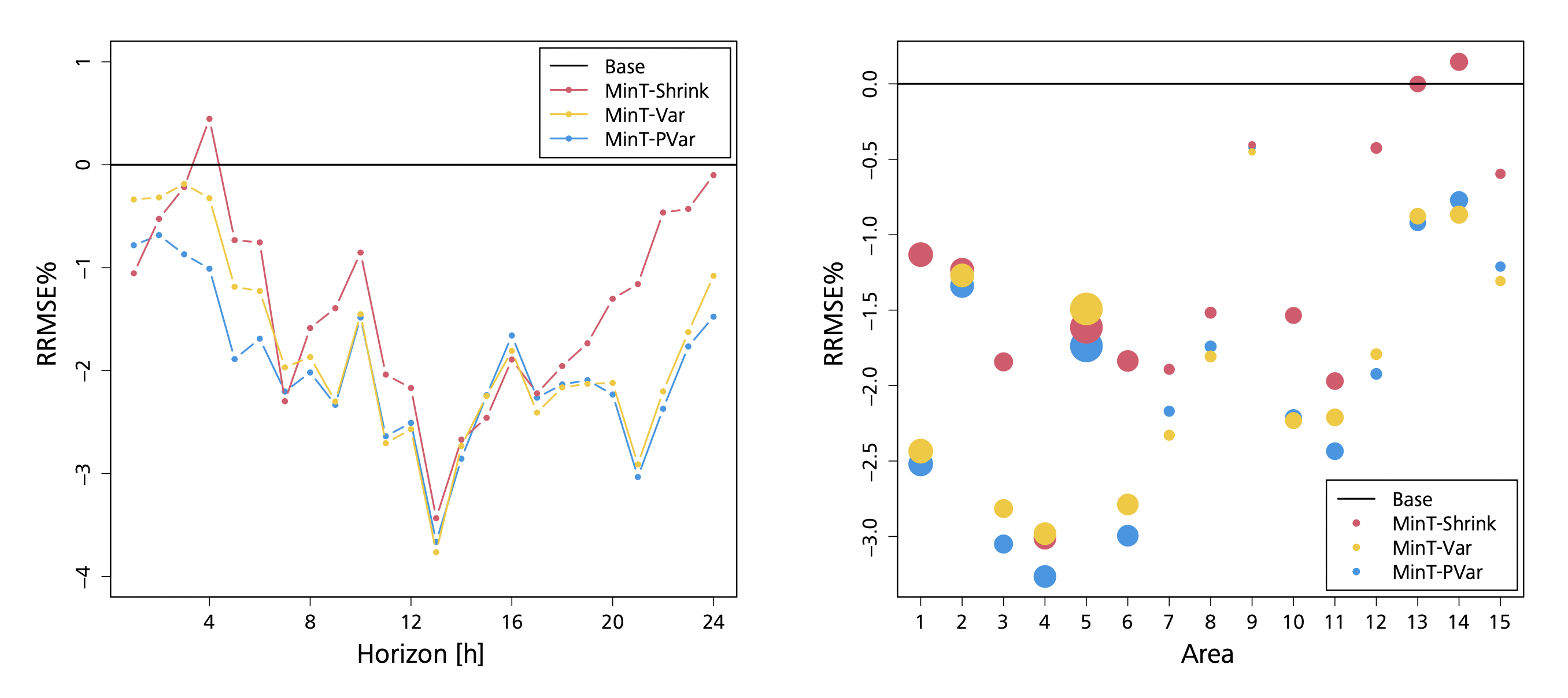
The three methods that have been tested are able to improve the accuracy of the base forecast across almost all horizons. Only MinT-Shrink falls below the base forecast in accuracy, and only for a single horizon. There seems to be a pattern to the accuracy improvements for all methods, where the RRMSE drops until the 13-hour horizon and then rises until the end of the 24-hour cycle.
Looking at how the methods perform for each area, MinT-Var and MinT-PVar once again come out as the best methods. In all areas tested, either MinT-Var or MinT-PVar had the best performance. MinT-Var falls behind MinT-Shrink in areas no. 4 and 5, while MinT-PVar is consistently better than MinT-Shrink. This highlights the importance of adapting the correlation to the forecast, as for some areas only adapting the variance is clearly not enough.
Altogether the results show that a reconciliation based on temporal hierarchies can improve even already state-of-the-art commercial wind power forecasts. Although the average improvement of approximately 2% does not seem like much, such improvements are still significant for what are already high-quality forecasts. Further applying the variance estimation techniques proposed in this study results in additional improvements in accuracy, especially when combined with the use of Pearson residuals for correlation estimation.
6 Discussion and conclusion
The investigations performed in this study have shown that, even when using rather simple base forecasts for all the aggregated levels, commercial state-of-the-art base forecasts can be improved using forecast reconciliation based on temporal hierarchies. This finding is very promising, as integrating the method of forecast reconciliation into commercial forecasts can thus help meet the demand for increasingly accurate forecasts. The additional coherency property will also be advantageous for the TSOs, as the planning across multiple time horizons becomes simpler and more coherent.
As discussed throughout the study, reconciling forecasts of wind power production poses some challenges in terms of the non-constant variance. The variance will depend greatly on, e.g., the wind speed. Introducing a method which adapts the variance structure to the weather forecast thus helps in addressing this challenge. This more rigorous approach to reconciliation reflecting the conditional variance dependency on the prediction has resulted in better accuracy of the reconciled forecast.
For cases from other fields where data are close to Gaussian, it is more reasonable to assume that the covariance is constant or at least independent of the mean. Hence, we expect less difference between our proposed method and the MinT-Shrink in these cases.
There is, however, still much that can be done to build upon the results found here, and as such these results can be seen as a step towards an improved methodology for modelling the required covariance structure for reconciling forecasts in cases with non-constant variance. Furthermore, this can help build toward a more general understanding of the uncertainty in forecasts when using hierarchies.
Other authors have also developed methods for handling, e.g., bounded data [18 S. L. Wickramasuriya, B. A. Turlach and R. J. Hyndman, Optimal non-negative forecast reconciliation. Stat. Comput. 30, 1167–1182 (2020) ]. It would therefore be interesting to examine how this performs compared to our proposed adjustments, or if these methods could be combined in a meaningful way. Due to the limits imposed by the data in this study, further testing on different data would also be beneficial to more confidently show which method is preferable when reconciling forecasts of wind power production.
Acknowledgements. We extend a sincere thank you to Krzysztof Burnecki for kindly inviting us to write this article.
Funding. This work is supported by SEM4Cities (Innovation Fund Denmark, no. 0143-0004), ARV (H2020-101036723), ELEXIA (EU HE-101075656), IEA Wind Task 51 (EUDP nr. 134-22015), and finally the projects PtX, Sector Coupling and LCA and DynFlex, which both are part of the Danish Mission Green Fuel portfolio of projects.
- 1
IRENA, Global energy transformation: A roadmap to 2050; https://www.irena.org/publications/2019/Apr/Global-energy-transformation-A-roadmap-to-2050-2019Edition.
- 2
References
- G. Athanasopoulos, R. A. Ahmed and R. J. Hyndman, Hierarchical forecasts for Australian domestic tourism. Int. J. Forecast. 25, 146–166 (2009)
- G. Athanasopoulos, R. J. Hyndman, N. Kourentzes and F. Petropoulos, Forecasting with temporal hierarchies. Eur. J. Oper. Res. 262, 60–74 (2017)
- H. G. Bergsteinsson, J. K. Møller, P. Nystrup, Ó. P. Pálsson, D. Guericke and H. Madsen, Heat load forecasting using adaptive temporal hierarchies. Appl. Energ. 292, article no. 116872 (2021)
- F. Cribari-Neto and A. Zeileis, Beta regression in R. J. Stat. Software 34, 1–24 (2010)
- C. Di Modica, P. Pinson and S. Ben Taieb, Online forecast reconciliation in wind power prediction. Electr. Power Syst. Res. 190, article no. 106637 (2021)
- M. E. Hansen, P. Nystrup, J. K. Møller and H. Madsen, Reconciliation of wind power forecasts in spatial hierarchies. Wind Energ. 26, 615–632 (2023)
- R. J. Hyndman, R. A. Ahmed, G. Athanasopoulos and H. L. Shang, Optimal combination forecasts for hierarchical time series. Comput. Statist. Data Anal. 55, 2579–2589 (2011)
- R. J. Hyndman, A. J. Lee and E. Wang, Fast computation of reconciled forecasts for hierarchical and grouped time series. Comput. Statist. Data Anal. 97, 16–32 (2016)
- N. Kourentzes and G. Athanasopoulos, Cross-temporal coherent forecasts for Australian tourism. Ann. Tourism Res. 75, 393–409 (2019)
- M. Lange, On the uncertainty of wind power predictions – Analysis of the forecast accuracy and statistical distribution of errors. J. Sol. Energ. Eng. 127, 177–184 (2005)
- H. Madsen and P. Thyregod, Introduction to general and generalized linear models. CRC Press, Boca Raton, FL (2011)
- J. K. Møller, M. Zugno and H. Madsen, Probabilistic forecasts of wind power generation by stochastic differential equation models. J. Forecast. 35, 189–205 (2016)
- H. A. Nielsen, H. Madsen and T. S. Nielsen, Using quantile regression to extend an existing wind power forecasting system with probabilistic forecasts. Wind Energ. 9, 95–108 (2006)
- P. Nystrup, E. Lindström, P. Pinson and H. Madsen, Temporal hierarchies with autocorrelation for load forecasting. Eur. J. Oper. Res. 280, 876–888 (2020)
- P. Pinson, Wind energy: Forecasting challenges for its operational management. Stat. Sci. 28, 564–585 (2013)
- M. L. Sørensen, P. Nystrup, M. B. Bjerregård, J. K. Møller, P. Bacher and H. Madsen, Recent developments in multivariate wind and solar power forecasting. WIREs Energy Environ. 12, article no. e465 (2023)
- S. L. Wickramasuriya, G. Athanasopoulos and R. J. Hyndman, Optimal forecast reconciliation for hierarchical and grouped time series through trace minimization. J. Am. Stat. Assoc. 114, 804–819 (2019)
- S. L. Wickramasuriya, B. A. Turlach and R. J. Hyndman, Optimal non-negative forecast reconciliation. Stat. Comput. 30, 1167–1182 (2020)
Cite this article
Mikkel L. Sørensen, Jan K. Møller, Henrik Madsen, Reconciling temporal hierarchies of wind power production with forecast-dependent variance structures. Eur. Math. Soc. Mag. 130 (2023), pp. 4–13
DOI 10.4171/MAG/172