
The recent frantic surge of machine learning and, more broadly, of artificial intelligence (AI) brings to light old and new open issues, and among them, the so-called eXplainable artificial intelligence (XAI) – AI that humans can understand – as opposed to black-box learning systems where even their designers cannot explain AI decisions. One of the major XAI questions is how to design transparent learning systems that incorporate prior knowledge. These topics are becoming more relevant and pervasive as AI systems become more unfathomable and entangled with human factors. Recently a new paradigm for XAI has been introduced in literature, based on group equivariant non-expansive operators (GENEOs), which are able to inject prior knowledge in a learning system. Hence, the use of GENEOs dramatically reduces the number of unknown parameters to be identified and the size of the related training set, providing both computational advantages and an increased degree of interpretability of the results. Here we will illustrate the main characteristics of GENEOs and the encouraging results already obtained on a couple of industrial case studies.
1 Introduction
The use of techniques and architectures of artificial intelligence (AI) is becoming more and more pervasive in a wide range of applications, starting from automation or quality control in industry, to self-driving vehicles, crime surveillance, health monitoring and many others.
As the Oxford Dictionary states, by AI one means the theory and development of computer systems able to perform tasks normally requiring human intelligence, such as visual perception, speech recognition, decision-making, and translation between languages. Such systems are quite often based on machine or deep learning techniques, that is, on different types of neural networks, with many layers and thus with a huge number of unknown parameters, which need to be identified on the basis of a training set of data. Even if in many applications AI and deep learning prove to be very effective, two main problems often arise: the limited availability of data in some applications, which prevents the scientists to define a sufficiently large training set, and the ‘black-box’ nature of deep learning systems, having as a consequence that even its designers cannot explain AI decisions.
Equivariant operators are proving to be increasingly important in deep learning, in order to make neural networks more transparent and interpretable [2 F. Anselmi, G. Evangelopoulos, L. Rosasco and T. Poggio, Symmetry-adapted representation learning. Pattern Recognition 86, 201–208 (2019) , 3 F. Anselmi, L. Rosasco and T. Poggio, On invariance and selectivity in representation learning. Inf. Inference 5, 134–158 (2016) , 4 Y. Bengio, A. Courville and P. Vincent, Representation learning: A review and new perspectives. IEEE Trans. Pattern Anal. Mach. Intell. 35, 1798–1828 (2013) , 10 T. Cohen and M. Welling, Group equivariant convolutional networks. In International Conference on Machine Learning, 2990–2999 (2016) , 20 S. Mallat, Group invariant scattering. Comm. Pure Appl. Math. 65, 1331–1398 (2012) , 21 S. Mallat, Understanding deep convolutional networks. Philos. Trans. R. Soc. Lond., A 374, article no. 20150203 (2016) , 27 D. E. Worrall, S. J. Garbin, D. Turmukhambetov and G. J. Brostow, Harmonic networks: Deep translation and rotation equivariance. In Proc. IEEE Conf. on Computer Vision and Pattern Recognition (CVPR), 7168–7177 (2017) , 28 C. Zhang, S. Voinea, G. Evangelopoulos, L. Rosasco and T. Poggio, Discriminative template learning in group-convolutional networks for invariant speech representations. In INTERSPEECH-2015, International Speech Communication Association, Dresden, Germany, 3229–3233, (2015) ]. The use of such operators corresponds to the rising interest in the so-called “explainable machine learning” [8 A. P. Carrieri, N. Haiminen, S. Maudsley-Barton, L.-J. Gardiner, B. Murphy, A. E. Mayes, S. Paterson, S. Grimshaw, M. Winn, C. Shand, P. Hadjidoukas, W. P. M. Rowe, S. Hawkins, A. MacGuire-Flanagan, J. Tazzioli, J. G. Kenny, L. Parida, M. Hoptroff and E. O. Pyzer-Knapp, Explainable AI reveals changes in skin microbiome composition linked to phenotypic differences. Sci. Rep. 11, article no. 4565 (2021) , 14 S. A. Hicks, J. L. Isaksen, V. Thambawita, J. Ghouse, G. Ahlberg, A. Linneberg, N. Grarup, I. Strümke, C. Ellervik, M. S. Olesen, T. Hansen, C. Graff, N.-H. Holstein-Rathlou, P. Halvorsen, M. M. Maleckar, M. A. Riegler and J. K. Kanters, Explaining deep neural networks for knowledge discovery in electrocardiogram analysis. Sci. Rep. 11, article no. 10949 (2021) , 23 C. Rudin, Stop explaining black box machine learning models for high stakes decisions and use interpretable models instead. Nat. Mach. Intell. 1, 206–215 (2019) ], which looks for methods and techniques that can be understood by humans. In accordance with this line of research, group equivariant non-expansive operators (GENEOs) have been recently proposed as elementary components for building new kinds of neural networks [5 M. G. Bergomi, P. Frosini, D. Giorgi and N. Quercioli, Towards a topological-geometrical theory of group equivariant non-expansive operators for data analysis and machine learning. Nat. Mach. Intell. 1, 423–433 (2019) , 6 G. Bocchi, S. Botteghi, M. Brasini, P. Frosini and N. Quercioli, On the finite representation of group equivariant operators via permutant measures. Ann. Math. Artif. Intell. DOI 10.1007/s10472-022-09830-1 (2023) , 11 F. Conti, P. Frosini and N. Quercioli, On the construction of group equivariant non-expansive operators via permutants and symmetric functions. Front. Artif. Intell. Appl. 5, DOI 10.3389/frai.2022.786091 (2022) ]. Their use is grounded in topological data analysis (TDA) and guarantees good mathematical properties, such as compactness, convexity, and finite approximability, under suitable assumptions on the space of data and by choosing appropriate topologies. Furthermore, GENEOs allow to shift the attention from the data to the observers who process them, and to incorporate the properties of invariance and simplification that characterize those observers. The basic idea is that we are not usually interested in data, but in approximating the experts’ opinion in presence of the given data [12 P. Frosini, Towards an observer-oriented theory of shape comparison: Position paper. In Proceedings of the Eurographics 2016 Workshop on 3D Object Retrieval, Eurographics Association, Goslar, 5-–8 (2016) ].
More formally, a GENEO is a functional operator that transforms data into other data. By definition, it is assumed to commute with the action of given groups of transformations (equivariance) and to make the distance between data decrease (non-expansivity). The groups represent the transformations that preserve the “shape” of our data, while the non-expansivity condition means that the operator must simplify the data metric structure. Both equivariance and non-expansivity are important: while equivariance reduces the computational complexity by expressing the equivalence of data, non-expansivity guarantees that the space of GENEOs can be finitely approximated, under suitable assumptions. The key point for the use of GENEOs is the possibility of focusing on them in the search for optimal components of neural networks, instead of exploring the infinite-dimensional spaces of all possible operators. The relatively small dimension of the spaces of GENEOs – and their good geometric and topological properties – open the way to a new kind of “geometric knowledge engineering for deep learning,” which can allow us to drastically reduce the number of involved parameters and to increase the transparency of neural networks, by inserting information in the agents that are responsible for data processing.
In this paper we will introduce GENEOs and their main mathematical properties and we will show the quite promising results already obtained by their application to two different industrial problems, namely, protein pocket detection and maintenance of electric power lines.
Let us remark that, in rapidly evolving scientific fields like artificial intelligence, which claims for new ideas and mathematical instruments, it is crucial to establish a strict interaction and collaboration between academic mathematical research and industry, in order to focus on the most important mathematical problems that must be addressed to produce technological innovation. Such industry-academia interactions are fostered since many years by the European Consortium for Mathematics in Industry (ECMI)1https://ecmiindmath.org, with its many initiatives, and in particular with its biannual conference, whose next edition2https://ecmi2023.org will be held in Wrocław (Poland) on June 26–30, 2023.
2 GENEOs as models for observers
Observers can be often seen as functional operators, transforming data into other data. This happens, for example, when we blur an image by a convolution, or when we summarize data by descriptive statistics. However, observers are far from being entities that merely change functions into other functions. They do that in a compatible way with respect to some group of transformations, i.e., they commute with these transformations. For example, the operator associating to each regular function its Laplacian commutes with all Euclidean isometries of . More precisely, we say that this operator is equivariant with respect to the group of isometries.
Another important property of observers should also be considered: they are endowed with some kind of regularity. A particularly important regularity property is non-expansivity. That means that the distance between the input data is not smaller than the distance between the output functions. This type of regularity is frequently found in applications, since usually operators are required to simplify the metric structure of data. We can obviously imagine particular applications where this condition is violated locally, but the usual long term purpose of data processing is to converge to an interpretation, i.e., a representation that is much simpler and meaningful than the original data. As a consequence, it is reasonable to assume that the operators representing observers, as well as their iterated composition, are non-expansive. This assumption is not only useful for simplifying the analysis of data, but it is also fundamental in the proof that the space of group equivariant non-expansive operators is compact (and hence finitely approximable), provided that the space of data is compact with respect to a suitable topology [5 M. G. Bergomi, P. Frosini, D. Giorgi and N. Quercioli, Towards a topological-geometrical theory of group equivariant non-expansive operators for data analysis and machine learning. Nat. Mach. Intell. 1, 423–433 (2019) ].
2.1 Basic definitions and properties of GENEO spaces
Let us now formalize the concept of group-equivariant non-expansive operator, as was introduced in [5 M. G. Bergomi, P. Frosini, D. Giorgi and N. Quercioli, Towards a topological-geometrical theory of group equivariant non-expansive operators for data analysis and machine learning. Nat. Mach. Intell. 1, 423–433 (2019) ].
We assume that a space of functions from a set to is given, together with a group of transformations of , such that if and , then . We call the pair perception pair. We also assume that is endowed with the topology induced by the -distance , . Let us assume that another perception pair is given, with endowed with the topology induced by the analogous -distance , and let us fix a homomorphism .
Definition 1. A map is called a group equivariant non-expansive operator (GENEO) if the following conditions are satisfied:
for any and any (equivariance);
for any (non-expansivity).
If we denote by the space of all GENEOs between and and endow it with the metric
the following main properties of spaces of GENEOs hold true (see [5 M. G. Bergomi, P. Frosini, D. Giorgi and N. Quercioli, Towards a topological-geometrical theory of group equivariant non-expansive operators for data analysis and machine learning. Nat. Mach. Intell. 1, 423–433 (2019) ] for the proofs).
If and are compact, then is compact with respect to the topology induced by the metric .
Corollary 3. If and are compact with respect to the -metrics and , respectively, then for any the space can be -approximated by a finite set.
If is convex, then is convex.
Theorem 2 and Corollary 3 guarantee that if the spaces of data are compact, then also the space of GENEOs is compact, and can then be well approximated by a finite number of representatives, thereby reducing the complexity of the problem. Theorem 4 implies that if the space of data is also convex, then any convex combination of GENEOs is still a GENEO. Thus, when both compactness and convexity hold, we have an easy instrument to generate any element of starting from a finite number of operators. Additionally, the convexity of ensures that each strictly convex cost function in the space of the observers admits a unique minimum, and thus the problem of finding the ‘optimal observer’ can be solved.
3 Application to protein pockets detection: GENEOnet
We used GENEOs to build GENEOnet [7 G. Bocchi, P. Frosini, A. Micheletti, A. Pedretti, C. Gratteri, F. Lunghini, A. R. Beccari and C. Talarico, GENEOnet: A new machine learning paradigm based on group equivariant non-expansive operators. An application to protein pocket detection. arXiv:2202.00451 (2022) ], a geometrical machine-learning method able to detect pockets on the surface of proteins. Protein pockets detection is a key problem in the context of drug development, since the ability to identify only a small number of sites on the surface of a molecule that are good candidates to become binding sites allows a scientist to restrict the action of virtual screening procedures, thus saving both computational resources and time, and fostering the speed up of the subsequent phases of the process. This research is still ongoing, in collaboration with the Italian pharmaceutical company Dompé Farmaceutici.
This problem is particularly suitable to be treated with GENEOs, since, on the one hand, there is some important empirical chemical-physical knowledge that cannot be embedded in the usual machine learning techniques, but can be injected in a GENEO architecture, and, on the other hand, the problem enjoys a natural invariance property: indeed, if we rotate or translate a protein, its pockets will undergo the same transformation, coherently with the entire protein. This clearly implies that pocket detection is equivariant with respect to the group of spatial isometries.
For this application we used a subset of more than 10,000 protein-ligand complexes extracted from the PDBbind v2020 dataset [19 Z. Liu, M. Su, L. Han, J. Liu, Q. Yang, Y. Li and R. Wang, Forging the basis for developing protein-ligand interaction scoring functions. Acc. Chem. Res. 50, 302–309 (2017) ]. Input data was discretized by surrounding each molecule by a cubic bounded region divided into a 3D grid of voxels. In this way the data are modelled as bounded functions from the Euclidean space to . We chose , that is, the number of distinct geometrical, chemical and physical potential fields that we computed on each molecule and took into account for the analysis. The potentials are here called ‘channels’, imitating the nomenclature used in image analysis (see [7 G. Bocchi, P. Frosini, A. Micheletti, A. Pedretti, C. Gratteri, F. Lunghini, A. R. Beccari and C. Talarico, GENEOnet: A new machine learning paradigm based on group equivariant non-expansive operators. An application to protein pocket detection. arXiv:2202.00451 (2022) ] for further details on the specific channels).
3.1 The GENEOnet model
The input data are fed to a first layer of GENEOs chosen from a set of parametric families of operators, each one parametrized by one single shape parameter , . These families were designed in order to include the a priori knowledge of the experts of medicinal chemistry in the equivariance properties of the GENEOs. We opted for convolutional operators, whose properties can be completely determined by the nature of their convolution kernels. Moreover, by making the -th kernel dependent on only one shape parameter , we have direct control on the action of each operator. We mainly used Gaussian kernels or kernels having shapes of spheres or of spherical crowns, assuming alternatively positive and negative values in different parts of the interior of the sphere or crown, and zero outside. In this way we could detect both spherical voids close to the protein that are surrounded by protein atoms and the change of sign of the measured potentials, since protein cavities which show high gradients of the values of the measured potentials are the most promising to become binding sites. The shape parameter of each kernel was connected with the radius of the sphere or spherical crown, or with the standard deviation of the Gaussian.
All the chosen operators share a common feature: their kernels are defined through rotationally-invariant functions. This fact, together with the properties of convolution, guarantees that the corresponding GENEOs satisfy the key requirement to be equivariant with respect to the group of isometries of .
In the second step, these operators are combined through a convex combination with weights such that for all and . We then obtain a composite operator whose output is normalized to a function from to . Here can be interpreted as the probability that a point belongs to a pocket. Finally, given a probability threshold , we get the different pockets returned by the model by taking the connected components of the superlevel set . The entire model pipeline is depicted in Figure 1.

A discretization into voxels similar to the one adopted for the molecules has been applied also to the GENEOs, which have thus been expressed as discrete convolutional operators. The choice of convolutional operators allowed us to exploit the efficient implementation of discrete convolution, reducing the computational costs.
3.2 Parameter identification
The model that was described so far, as shown in Figure 1, has a total of 17 parameters (, , , and ). The codes were written using both C and Python. The fact that the model only employs convolutional operators and linear combinations thereof allowed us to set up an optimization pipeline quite similar to a 3D convolutional neural network (CNN), but with two fundamental differences. First, our model has a really tiny set of parameters, if compared to a classical CNN: we estimated that a recent method called DeepSite [15 J. Jimenez, S. Doerr, G. Martinez-Rosell, A. S. Rose and G. De Fabritiis, DeepSite: Protein-binding site predictor using 3D-convolutional neural networks. Bioinform. 33, 3036–3042 (2017) ], which implements a classical 3D CNN for pocket detection, has parameters; DeepPocket [1 R. Aggarwal, A. Gupta, V. Chelur, C. V. Jawahar and U. Deva Priyakumar, DeepPocket: Ligand binding site detection and segmentation using 3D convolutional neural networks. J. Chem. Inf. Model. DOI 10.26434/chemrxiv-2021-7fkkx-v2 (2021) ], an even newer approach that uses a 3D CNN to rescore fPocket [18 V. Le Guilloux, P. Schmidtke and P. Tuffery, Fpocket: An open source platform for ligand pocket detection. BMC Bioinform. 10, article no. 168 (2009) ] predictions, has parameters. Second, the convolutional kernels of the GENEOs are not learned entry by entry as in classical CNNs, since in this way equivariance would not be preserved at each iteration; instead, at each step the kernels are recomputed from the shape parameters that are updated during the optimization. Finally, the estimated values of the parameters , , can be interpreted as weights giving the relative importance of each considered channel to the final pocket detection.
In order to identify the unknown parameters, we have to optimize a cost function that evaluates the goodness of our predictions. If we denote by the output of the model after thresholding, then we must compare to the ground truth represented by the binary function , which takes the value 1 in those voxels occupied by the ligand and 0 in the other voxels. We adopted the following accuracy function that needs to be maximized:
Here denotes the minimum between the two functions, denotes the volume of the set where the function equals 1 and denotes the constant function equal to 1. Note that the function is well defined, since all our functions are defined only on a (voxelized) compact cubic region surrounding the molecule. The hyperparameter ranges in , and when , the accuracy function is simply the fraction of correctly labelled voxels out of the total. We choose , which allows to balance the two terms of the sum in the numerator to obtain more and slightly bigger pockets. In particular, we empirically found that values of in the interval give similar and good results, all characterized by a rather small number of pockets of suitable size.
Eventually, pockets are found as the connected components of the thresholded output of the model. In this way we get an array where voxels located in a pocket are labelled with the successive number of the connected component they belong to, while they are labelled with 0 if they do not belong to a pocket. Actually, this representation is not very informative, since in the applications of pocket detection in medicinal chemistry it is desirable to compute also the druggability of the identified cavities, that is, a ranking of the pockets on the basis of their fitness to host a ligand.
To assign a score to each pocket, we went back to the output of the model before the thresholding, that is, to the function , which was interpreted as the probability that a voxel belongs to a pocket. The score of a pocket was then computed as the average value of taken only over the voxels belonging to the pocket, rescaled by a factor proportional to the volume of the pocket so as to avoid giving too high scores to very small pockets. Eventually, the final output of the model consists in a list of pockets, given as the coordinates of their voxels, and the corresponding scores.
Figure 2 displays an example of results of GENEOnet applied to the protein 2QWE. The picture shows a relevant aspect of GENEOnet: the depicted protein is made up of four symmetrical units so that the true pocket is replicated four times. GENEOnet correctly outputs, among the others, four symmetrical pockets that receive high scores. This happens thanks to equivariance, because the results of the model on identical units are the same, with position and orientation coherently adjusted.
3.3 Comparison between GENEOnet and other methods
We compared the results of GENEOnet with a set of other recent methods for protein pocket detection based on machine learning techniques. Since the output of such methods can be different from our output, both in terms of the discretization strategy and of the objective function to be optimized, we decided to base our comparison on the scores given by the different methods to the cavities. In this way we can perform a comparison based on the ability of the model to assign the highest scores to pockets that match the true ones. Given our dataset of proteins, having only one ligand, and thus one ‘true pocket’ each, we can compute the fraction of proteins whose true pocket is hit by the predicted one with highest score, by the one with second highest score, and so on. We say that a predicted pocket hits the true pocket if has the greatest overlap with . If no predicted pocket has an intersection with the true one, we say that the method failed on that protein. Finally, we computed the cumulative sum of these fractions; in this way we get a curve where the -th point represents the fraction of proteins whose true pocket has been recognized within the first highest scored predicted pockets.
In the following we will denote by the proportion of correct recognitions, i.e.,
and by the corresponding cumulative quantities, i.e.,
In this way different methods can be compared directly: if a model has a cumulative curve that stands above all the others, then that model is definitely better. We chose to use this approach to compare our model with the following other state-of-the-art methods:
fPocket [16 R. Krivák and D. Hoksza, P2Rank: Machine learning based tool for rapid and accurate prediction of ligand binding sites from protein structure. J. Cheminform. 10 article no. 39 (2018) ]: a fast geometrical method that employs a detection algorithm based on alpha-spheres.
P2RANK [18 V. Le Guilloux, P. Schmidtke and P. Tuffery, Fpocket: An open source platform for ligand pocket detection. BMC Bioinform. 10, article no. 168 (2009) ]: a model that uses random forests to make predictions on a cloud of points evenly sampled on the solvent accessible surface.
DeepPocket [1 R. Aggarwal, A. Gupta, V. Chelur, C. V. Jawahar and U. Deva Priyakumar, DeepPocket: Ligand binding site detection and segmentation using 3D convolutional neural networks. J. Chem. Inf. Model. DOI 10.26434/chemrxiv-2021-7fkkx-v2 (2021) ]: a method that performs a re-scoring of fPocket cavities by means of 3D CNNs.
Caviar [22 J.-R. Marchand, B. Pirard, P. Ertl and F. Sirockin, CAVIAR: A method for automatic cavity detection, description and decomposition into subcavities. J. Comput. Aided Mol. Des. 35, 737–750 (2021) ]: a model that uses a novel approach to the classical technique of points enclosure.
SiteMap [13 T. Halgren, New method for fast and accurate binding-site identification and analysis. Chem. Biol. Drug. Des. 69, 146–148 (2007) ]: a model that clusterizes site points based on surface distance and how well they are sheltered from the solvent.
CavVis [24 T. M. C. Simoes and A. J. P. Gomes, CavVis. A field-of-view geometric algorithm for protein cavity detection. J. Chem. Inf. Model. 59, 786–796 (2019) ]: a model that uses Gaussian surfaces to predict pockets based on a visibility criterion.
The results are reported in Figure 3, which demonstrates that GENEOnet has a better performance than all the other methods considered in the comparison.
4 SCENE-net: application of GENEOs to LiDAR scans segmentation for maintenance of electric power plants
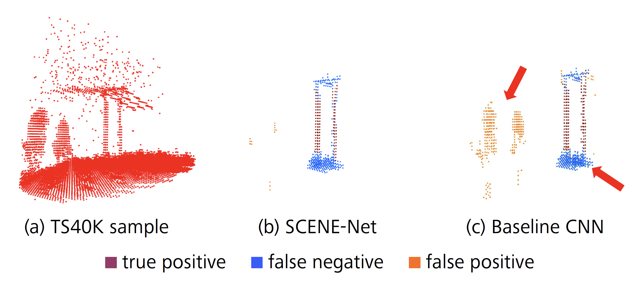
In Portugal, the maintenance and inspection of the energy transmission system is based on LiDAR point clouds. Low-flying helicopters are deployed to scan the environment from a bird-eye view (BEV) perspective and store the results in a 3D point cloud format for further processing by maintenance personnel. This results in detailed large-scale point clouds with high point density, no sparsity and no object occlusion. The captured 3D scenes are quite extensive and mostly composed of arboreal/rural areas, with the transmission line making a small percentage of the LiDAR scans. As a result, maintenance specialists spend the majority of their time manually sectioning and labelling 3D data in order to focus on 3D scenes that encompass the transmission line, for later inspection, to avoid collisions with the vegetation that may cause fires. In order to accelerate this task, we applied GENEOs to the detection of power-line supporting towers and produced a semantic segmentation. These metal structures serve as points of reference for the location of the electrical network. By doing so, the laborious task of manually searching and sectioning the 3D scenes that contain parts of the transmission network can be automated, which grants a significant speed-up to the whole procedure. This research is still going on and is performed in collaboration with the CNET Center for New Energy Technologies SA, of the company EDP, the main electric energy provider in Portugal.
We considered a dataset provided by EDP, using km of rural and forest terrain labelled with 22 classes, culminating in 2823 samples describing the transmission system, named TS40K (see Figure 4). Withal, the provided point clouds exhibit noisy labels and are mainly composed of non-relevant classes for our problem, such as the ground. Power-line supporting towers make up less than 1% of the overall point clouds, which makes noisy labelling a major issue for the segmentation task. For instance, patches of ground incorrectly classified as tower amount to roughly 40% of tower 3D points.
One plausible way to approach our problem would be to employ state-of-the-art methods with respect to 3D semantic segmentation. However, most proposals [9 R. Cheng, R. Razani, E. Taghavi, E. Li and B. Liu, (AF)2-S3NET: Attentive feature fusion with adaptive feature selection for sparse semantic segmentation network. In 2021 IEEE/CVF Conference on Computer Vision and Pattern Recognition (CVPR), 12542–12551 (2021) , 26 H. Thomas, C. Qi, J.-E. Deschaud, B. Marcotegui, F. Goulette and L. J. Guibas, KPConv: Flexible and deformable convolution for point clouds. In 2019 IEEE/CVF International Conference on Computer Vision (ICCV), 6410–6419 (2019) , 29 X. Zhu, H. Zhou, T. Wang, F. Hong, W. Li, Y. Ma, H. Li, R. Yang and D. Lin, Cylindrical and asymmetrical 3D convolution networks for LiDAS-based perception. IEEE Trans. Pattern Anal. Mach. Intell. 44, 6807–6822 (2021) ] do not account for the existence of ground, as it is usually removed to boost efficiency in urban settings, and this is not possible in rural scenes, due to their irregular terrain. Moreover, the high point density combined with the severe class imbalance and noisy labelling in TS40K are sure to affect the performance of these models in real scenarios.
We then built an architecture called SCENE-net, based on GENEOs [17 D. R. M. M. Lavado, Detection of power line supporting towers with group equivariant non-expansive operators. MSc thesis, NOVA University, Lisbon (2022) ], whose equivariance properties encode prior knowledge on the objects of interest (such as geometrical characteristics of towers) and embed them into a model still based on convolutional kernels, similarly to the previous application.
Note that also for this problem there is a piece of information that can be injected in a learning system based on GENEOs, exploiting the equivariance property. In fact, the shape of the towers could easily be recognized by a human being, but should be learned by a ‘blind’ machine-learning system. Therefore, also in this case study, the knowledge injection in the GENEO network results in a simplified and thus more interpretable model.
4.1 SCENE-net: the model
The pipeline used for SCENE-net is quite similar to the one of GENEOnet, used for protein pocket detection. A schematic representation is reported in Figure 5.
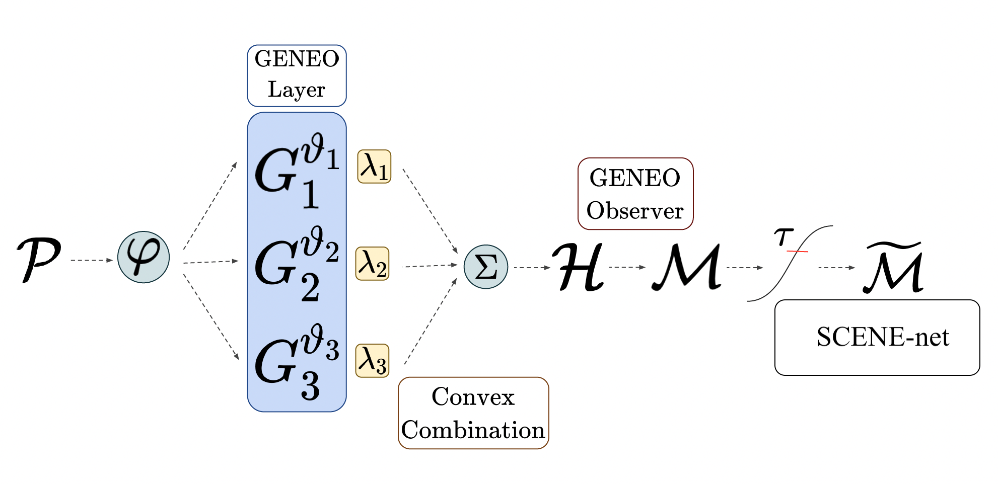
The input is a point cloud denoted by , where is the number of points and is the number of spatial coordinates and of any point-wise recorded features, such as colors, labels, normal vectors, etc. The cloud is first discretized, using a 3D regular grid, or voxel discretization of the considered scene, and then fed to a layer of GENEOs (GENEO layer), each chosen from a parametric family of operators, and defined by a set of trainable shape parameters , . Such GENEOs are employed as kernels for convolutional operators. The output of the GENEO layer is then combined into another GENEO obtained by a convex combination of the , with weights :
where is a point of the discretization grid. Because of the properties of GENEOs recalled in Section 2.1, is still a GENEO that can be interpreted as an ‘expert’ observer, and the estimated value of each coefficient represents the contribution given to the expert observer by the ‘naive observer’ . The parameters grant then our model its intrinsic interpretability. They are learned during training and represent the importance of each , and, by extension, the importance of their encoded properties, in modelling the ground truth.
Next, we transform the observer’s analysis into the probability that belongs to a supporting tower, as follows:
Negative signals in represent patterns that do not exhibit the sought-out geometrical properties. Conversely, positive values quantify their presence. Therefore, tanh compresses the observer’s value distribution into , and a rectified linear unit (ReLU) is then applied to enforce a zero probability to negative signals.
Lastly, a probability threshold is defined and applied to to detect the points of the discretization grid that lie on the towers:
In order to recognize the main geometrical characteristics of towers, we used three different kernels for the GENEOs :
A cylindrical kernel, with main axis orthogonal to the plane of the ground. The corresponding GENEO is thus equivariant under rotations around a vertical axis and is able to identify vertical structures which are much higher than the surrounding landscape, as towers are.
A cone-cylinder kernel, formed by a cylinder with a cone on the top. The corresponding GENEO is still equivariant under rotations around a vertical axis and is able to distinguish towers from trees, because of the typical shape formed by power lines stemming from the top of the towers.
A sphere with negative values in its interior, able to detect bushes and tree crowns and to assign them a negative weight.
4.2 Parameter identification
The unknown parameters , of the model are identified by solving the optimization problem
Here the loss is defined by
where is the estimated probability that the voxel lies on a tower, is the ground truth probability that voxel lies on a tower (computed as the proportion of LiDAR scanned points lying in voxel whose labels belong to a tower) and is a weight as proposed in [25 M. Steininger, K. Kobs, P. Davidson, A. Krause and A. Hotho, Density-based weighting for imbalanced regression. Mach. Learn. 110, 2187–2211 (2021) ] to mitigate data imbalance. The hyperparameter emphasizes the weighting scheme, whereas is a small positive number which ensures that the weights of the samples are positive (see [17 D. R. M. M. Lavado, Detection of power line supporting towers with group equivariant non-expansive operators. MSc thesis, NOVA University, Lisbon (2022) , 25 M. Steininger, K. Kobs, P. Davidson, A. Krause and A. Hotho, Density-based weighting for imbalanced regression. Mach. Learn. 110, 2187–2211 (2021) ] for more details).
Like in the previous case study, the Adam algorithm was applied to solve the optimization problem.
4.3 SCENE-net results and comparison with other methods
In order to limit the unbalanced nature of the dataset in the training phase, the entire TS40K dataset has been sectioned into 2823 subsets, each cropped around one different supporting tower. The samples have then been randomly split into a training set (80% of the total), a validation set (20% of the total), and a test set (10% of the total).
The results of SCENE-net have been compared with those of a convolutional neural network (CNN) applied to the same data. The following metrics have been used to compare the two methods:
Precision = (# true positive)/(# true positive + # false positive). This index tells us from all voxels predicted positively, what percentage did the model classify correctly.
Recall = (# true positive)/(# true positive + # false negative). This index provides the percentage of voxels lying on a tower that were correctly classified.
Intersection over union (IoU) = (# true positive)/(# true positive + # false negative + # false positive). This index measures the overlap between the prediction and the ground truth, over the total volume they occupy.
The results are reported in Table 1.
| Method | Precision | Recall | IoU |
| CNN | () | () | |
| SCENE-net | () | () |
Quantitatively, using SCENE-net we observe a lift in Precision of 24%, and of 5% in IoU, and a drop of 10% in Recall. The lower Recall of SCENE-Net is due to noisy labels in the ground truth. As shown in Figure 6, the ground surrounding supporting towers as well as power lines are often mislabeled as tower.
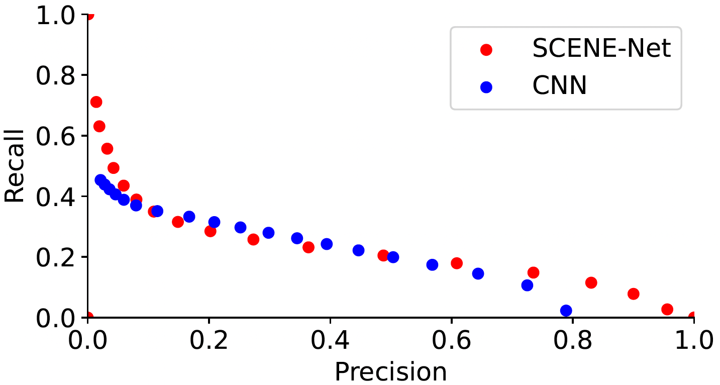
Additionally, from Figure 7 we note that the performance of SCENE-net is comparable to that of CNN when we change the classification threshold in the model pipeline, but SCENE-net has in total 11 parameters to be identified, while CNN has about unknown parameters and therefore needs to be trained with a much bigger training set.
Acknowledgements. Thanks to Krzysztof Burnecki for the kind invitation to write this article. Fruitful discussions and scientific collaborations on the subject of the article are also acknowledged to Patrizio Frosini (University of Bologna), Claudia Soares (NOVA University of Lisbon), and to Giovanni Bocchi and Diogo Lavado, who are the PhD students in Milan acting as driving force of this research. The author is also indebted to Alessandro Pedretti (Department of Pharmaceutical Sciences at University of Milan) for the interdisciplinary communication environment that initiated this work, and to the collaborators from EDP CNET Centre (Manuel Pio Silva, Alex Coronati) and from Dompé Farmaceutici (Andrea Beccari, Filippo Lunghini, Carmen Gratteri, Carmine Talarico), whose experience and attitude to interdisciplinary and cross-sectoral collaboration is a strong added value to this research. This work has been partially funded by Dompé Farmaceutici, and the collaboration started during events funded by the EU funded MSCA project BIGMATH (grant number 812912).
References
- R. Aggarwal, A. Gupta, V. Chelur, C. V. Jawahar and U. Deva Priyakumar, DeepPocket: Ligand binding site detection and segmentation using 3D convolutional neural networks. J. Chem. Inf. Model. DOI 10.26434/chemrxiv-2021-7fkkx-v2 (2021)
- F. Anselmi, G. Evangelopoulos, L. Rosasco and T. Poggio, Symmetry-adapted representation learning. Pattern Recognition 86, 201–208 (2019)
- F. Anselmi, L. Rosasco and T. Poggio, On invariance and selectivity in representation learning. Inf. Inference 5, 134–158 (2016)
- Y. Bengio, A. Courville and P. Vincent, Representation learning: A review and new perspectives. IEEE Trans. Pattern Anal. Mach. Intell. 35, 1798–1828 (2013)
- M. G. Bergomi, P. Frosini, D. Giorgi and N. Quercioli, Towards a topological-geometrical theory of group equivariant non-expansive operators for data analysis and machine learning. Nat. Mach. Intell. 1, 423–433 (2019)
- G. Bocchi, S. Botteghi, M. Brasini, P. Frosini and N. Quercioli, On the finite representation of group equivariant operators via permutant measures. Ann. Math. Artif. Intell. DOI 10.1007/s10472-022-09830-1 (2023)
- G. Bocchi, P. Frosini, A. Micheletti, A. Pedretti, C. Gratteri, F. Lunghini, A. R. Beccari and C. Talarico, GENEOnet: A new machine learning paradigm based on group equivariant non-expansive operators. An application to protein pocket detection. arXiv:2202.00451 (2022)
- A. P. Carrieri, N. Haiminen, S. Maudsley-Barton, L.-J. Gardiner, B. Murphy, A. E. Mayes, S. Paterson, S. Grimshaw, M. Winn, C. Shand, P. Hadjidoukas, W. P. M. Rowe, S. Hawkins, A. MacGuire-Flanagan, J. Tazzioli, J. G. Kenny, L. Parida, M. Hoptroff and E. O. Pyzer-Knapp, Explainable AI reveals changes in skin microbiome composition linked to phenotypic differences. Sci. Rep. 11, article no. 4565 (2021)
- R. Cheng, R. Razani, E. Taghavi, E. Li and B. Liu, (AF)2-S3NET: Attentive feature fusion with adaptive feature selection for sparse semantic segmentation network. In 2021 IEEE/CVF Conference on Computer Vision and Pattern Recognition (CVPR), 12542–12551 (2021)
- T. Cohen and M. Welling, Group equivariant convolutional networks. In International Conference on Machine Learning, 2990–2999 (2016)
- F. Conti, P. Frosini and N. Quercioli, On the construction of group equivariant non-expansive operators via permutants and symmetric functions. Front. Artif. Intell. Appl. 5, DOI 10.3389/frai.2022.786091 (2022)
- P. Frosini, Towards an observer-oriented theory of shape comparison: Position paper. In Proceedings of the Eurographics 2016 Workshop on 3D Object Retrieval, Eurographics Association, Goslar, 5-–8 (2016)
- T. Halgren, New method for fast and accurate binding-site identification and analysis. Chem. Biol. Drug. Des. 69, 146–148 (2007)
- S. A. Hicks, J. L. Isaksen, V. Thambawita, J. Ghouse, G. Ahlberg, A. Linneberg, N. Grarup, I. Strümke, C. Ellervik, M. S. Olesen, T. Hansen, C. Graff, N.-H. Holstein-Rathlou, P. Halvorsen, M. M. Maleckar, M. A. Riegler and J. K. Kanters, Explaining deep neural networks for knowledge discovery in electrocardiogram analysis. Sci. Rep. 11, article no. 10949 (2021)
- J. Jimenez, S. Doerr, G. Martinez-Rosell, A. S. Rose and G. De Fabritiis, DeepSite: Protein-binding site predictor using 3D-convolutional neural networks. Bioinform. 33, 3036–3042 (2017)
- R. Krivák and D. Hoksza, P2Rank: Machine learning based tool for rapid and accurate prediction of ligand binding sites from protein structure. J. Cheminform. 10 article no. 39 (2018)
- D. R. M. M. Lavado, Detection of power line supporting towers with group equivariant non-expansive operators. MSc thesis, NOVA University, Lisbon (2022)
- V. Le Guilloux, P. Schmidtke and P. Tuffery, Fpocket: An open source platform for ligand pocket detection. BMC Bioinform. 10, article no. 168 (2009)
- Z. Liu, M. Su, L. Han, J. Liu, Q. Yang, Y. Li and R. Wang, Forging the basis for developing protein-ligand interaction scoring functions. Acc. Chem. Res. 50, 302–309 (2017)
- S. Mallat, Group invariant scattering. Comm. Pure Appl. Math. 65, 1331–1398 (2012)
- S. Mallat, Understanding deep convolutional networks. Philos. Trans. R. Soc. Lond., A 374, article no. 20150203 (2016)
- J.-R. Marchand, B. Pirard, P. Ertl and F. Sirockin, CAVIAR: A method for automatic cavity detection, description and decomposition into subcavities. J. Comput. Aided Mol. Des. 35, 737–750 (2021)
- C. Rudin, Stop explaining black box machine learning models for high stakes decisions and use interpretable models instead. Nat. Mach. Intell. 1, 206–215 (2019)
- T. M. C. Simoes and A. J. P. Gomes, CavVis. A field-of-view geometric algorithm for protein cavity detection. J. Chem. Inf. Model. 59, 786–796 (2019)
- M. Steininger, K. Kobs, P. Davidson, A. Krause and A. Hotho, Density-based weighting for imbalanced regression. Mach. Learn. 110, 2187–2211 (2021)
- H. Thomas, C. Qi, J.-E. Deschaud, B. Marcotegui, F. Goulette and L. J. Guibas, KPConv: Flexible and deformable convolution for point clouds. In 2019 IEEE/CVF International Conference on Computer Vision (ICCV), 6410–6419 (2019)
- D. E. Worrall, S. J. Garbin, D. Turmukhambetov and G. J. Brostow, Harmonic networks: Deep translation and rotation equivariance. In Proc. IEEE Conf. on Computer Vision and Pattern Recognition (CVPR), 7168–7177 (2017)
- C. Zhang, S. Voinea, G. Evangelopoulos, L. Rosasco and T. Poggio, Discriminative template learning in group-convolutional networks for invariant speech representations. In INTERSPEECH-2015, International Speech Communication Association, Dresden, Germany, 3229–3233, (2015)
- X. Zhu, H. Zhou, T. Wang, F. Hong, W. Li, Y. Ma, H. Li, R. Yang and D. Lin, Cylindrical and asymmetrical 3D convolution networks for LiDAS-based perception. IEEE Trans. Pattern Anal. Mach. Intell. 44, 6807–6822 (2021)
Cite this article
Alessandra Micheletti, A new paradigm for artificial intelligence based on group equivariant non-expansive operators. Eur. Math. Soc. Mag. 128 (2023), pp. 4–12
DOI 10.4171/MAG/133