Solved and unsolved problems

The present column is devoted to Number Theory.

I Six new problems – solutions solicited

Solutions will appear in a subsequent issue.

269

Consider two positive integers $n\geq 1$ and $a\geq 2$ such that

is a prime. Prove that $n$ is a power of $3$.

Dorin Andrica and George Cătălin Ţurcaş (Babeş-Bolyai University, Cluj-Napoca, Romania)

270

The Collatz map is defined as follows:

Let

That is, $t_{m,x}$ is the smallest integer such that, if we apply the Collatz map $m$ times, the result is larger than $x$.

(a) Find $t_{3,1000}$ and $t_{4,1000}$.

(b) Show that, for $x$ large enough (larger than (say) $1000$), we have

(c) In general, for $m$ odd and $x$ large enough, there exists a constant $X_{m,x}$ such that $t_{m,x}$ is the smallest $n>X_{m,x}$ such that $n\equiv c_{m}\bmod M_{m}$. Find $M_{m}$ and relate $c_{m}$ to $c_{m-1}$.

Christopher Lutsko (Department of Mathematics, Rutgers University, Piscataway, USA)

271

The light-bulb problem: Alice and Bob are in jail for trying to divide by $0$. The jailer proposes the following game to decide their freedom: Alice will be shown an $n\times n$ grid of light bulbs. The jailer will point to a light bulb of his choice and Alice will decide whether it should be on or off. Then the jailer will point to another bulb of his choice and Alice will decide on/off. This continues until the very last bulb, when the jailer will decide whether this bulb is on or off. So the jailer controls the order of the selection, and the state of the final bulb. Alice is now removed from the room, and Bob is brought in. Bob’s goal is to choose $n$ bulbs such that his selection includes the final bulb (the one determined by the jailer).

Is there a strategy that Alice and Bob can use to guarantee success? What if Bob does not know the orientation in which Alice saw the board (i.e., what if Bob does not know which are the rows and which are the columns)?

Christopher Lutsko (Department of Mathematics, Rutgers University, Piscataway, USA)

272

Let $p$ and $q$ be coprime integers greater than or equal to $2$. Let $\operatorname{inv}_{q}(p)$ and $\operatorname{inv}_{p}(q)$ denote the modular inverse of $p\bmod q$ and $q\bmod p$, respectively. That is, $\operatorname{inv}_{q}(p)p\equiv 1\bmod q$ and $\operatorname{inv}_{p}(q)q\equiv 1\bmod p$.

(a) Show that

(b) Show by providing an example that, if $1\leq u<v$ are coprime integers and $\alpha≔u/v$, then the statement

is not necessarily true.

(c) What additional assumption should $p$ and/or $q$ satisfy so that the equivalence (⁠1⁠) holds?

Athanasios Sourmelidis (Institut für Analysis und Zahlentheorie, Technische Universität Graz, Austria)

273

Let $c_{n}(k)$ denote the Ramanujan sum defined as the sum of $k$th powers of the primitive $n$th roots of unity. Show that, for any integer $m\geq 1$,

where the sum is over all ordered pairs $(n,k)$ of positive integers $n,k$ such that their lcm is $m$, and $\varphi$ is Euler’s totient function.

László Tóth (University of Pécs, Hungary)

274

Show that, for every integer $n\geq 1$, we have the polynomial identity

where $\Phi_{d}(x)$ are the cyclotomic polynomials and $\varphi$ denotes Euler’s totient function.

László Tóth (Department of Mathematics, University of Pécs, Hungary)

II Open problem

275*. Chowla’s conjecture and its relatives

by Terence Tao (UCLA, Department of Mathematics, Los Angeles, USA)

Let $\lambda\colon\mathbb{N}\to\{-1,+1\}$ denote the Liouville function. In [⁠2⁠ S. Chowla, The Riemann hypothesis and Hilbert’s tenth problem. Mathematics and its Applications 4, Gordon and Breach Science Publishers, New York (1965) ], Chowla conjectured that

as $x\to\infty$, for any distinct natural numbers $h_{1},\ldots,h_{k}$ (in fact, Chowla made the more general conjecture that

whenever $P$ is a square-free polynomial mapping from $\mathbb{N}$ to $\mathbb{N}$). Chowla’s conjecture was extended to other bounded multiplicative functions by Elliott [⁠3⁠ P. D. T. A. Elliott, On the correlation of multiplicative functions. Notas Soc. Mat. Chile 11, 1–11 (1992) ] (see also a technical correction to the conjecture in [⁠8⁠ K. Matomäki, M. Radziwiłł and T. Tao, An averaged form of Chowla’s conjecture. Algebra Number Theory 9, 2167–2196 (2015) ]).

One can view (⁠2⁠) as a less difficult cousin of the notorious Hardy–Littlewood prime tuples conjecture [⁠4⁠ G. H. Hardy and J. E. Littlewood, Some problems of ‘Partitio numerorum’; III: On the expression of a number as a sum of primes. Acta Math. 44, 1–70 (1923) ], which conjectures an asymptotic of the form

where the singular series$\mathfrak{S}$ is an explicit product over primes of factors involving the numbers $h_{1},\ldots,h_{k}$. For $k=1$, both conjectures follow readily from the prime number theorem, but they remain open for higher $k$. However, the analogue of (⁠2⁠) (and (⁠3⁠) for $k\leq 2$) were recently established in certain function fields [⁠11⁠ W. Sawin and M. Shusterman, On the Chowla and twin primes conjectures over 𝔽q⁢[T]. Ann. of Math. (2) 196, 457–506 (2022) ], and are also known to hold in the presence of a Siegel zero [⁠1⁠ J. Chinis, Siegel zeros and Sarnak’s conjecture, preprint, arXiv:2105.14653 (2021) , ⁠5⁠ D. R. Heath-Brown, Prime twins and Siegel zeros. Proc. London Math. Soc. (3) 47, 193–224 (1983) , ⁠15⁠ T. Tao, J. Teräväinen, The Hardy–Littlewood–Chowla conjecture in the presence of a Siegel zero, preprint, arXiv:2109.06291 (2021) , ⁠6⁠ K. Matomäki, J. Merikoski, Siegel zeros, twin primes, Goldbach’s conjecture, and primes in short intervals, preprint, arXiv:2112.11412 (2021) ]. The conjecture (⁠2⁠) is also known if one performs enough averaging in the $h_{1},\dots,h_{k}$ variables [⁠8⁠ K. Matomäki, M. Radziwiłł and T. Tao, An averaged form of Chowla’s conjecture. Algebra Number Theory 9, 2167–2196 (2015) ].

The logarithmically averaged version

turns out to be more tractable, as it can be analyzed by the “entropy decrement method” [⁠12⁠ T. Tao, The logarithmically averaged Chowla and Elliott conjectures for two-point correlations. Forum Math. Pi 4, Paper No. e8 (2016) ], which has been successfully used to establish the conjecture for $k=2$ (see [⁠12⁠ T. Tao, The logarithmically averaged Chowla and Elliott conjectures for two-point correlations. Forum Math. Pi 4, Paper No. e8 (2016) ], building upon the breakthrough work [⁠7⁠ K. Matomäki and M. Radziwiłł, Multiplicative functions in short intervals. Ann. of Math. (2) 183, 1015–1056 (2016) ]) and for odd $k$ (see [⁠14⁠ T. Tao and J. Teräväinen, Odd order cases of the logarithmically averaged Chowla conjecture. J. Théor. Nombres Bordeaux 30, 997–1015 (2018) , ⁠16⁠ T. Tao and J. Teräväinen, The structure of logarithmically averaged correlations of multiplicative functions, with applications to the Chowla and Elliott conjectures. Duke Math. J. 168, 1977–2027 (2019) ]). The conjecture (⁠4⁠) for arbitrary $k$ is also known to be equivalent [⁠13⁠ T. Tao, Equivalence of the logarithmically averaged Chowla and Sarnak conjectures. In Number Theory—Diophantine Problems, Uniform Distribution and Applications, Springer, Cham, 391–421 (2017) ] to the (logarithmically averaged) Sarnak conjecture [⁠10⁠ P. Sarnak, Mobius randomness and dynamics. Not. S. Afr. Math. Soc. 43, 89–97 (2012) ], which asserts that

whenever $T\colon X\to X$ is a compact dynamical system of zero entropy, $x_{0}$ is a point in $X$, and $F\colon X\to\mathbb{C}$ is continuous. Many special cases of this conjecture are known, unfortunately too many to list here.

The conjecture (⁠4⁠) would also follow from a higher-order local Fourier uniformity conjecture [⁠12⁠ T. Tao, The logarithmically averaged Chowla and Elliott conjectures for two-point correlations. Forum Math. Pi 4, Paper No. e8 (2016) ], which is somewhat complicated to state in full generality here; however, the first unsolved special case of this conjecture asserts that

whenever $1\leq H=H(X)\leq X$ is such that $H(X)\to\infty$ as $X\to\infty$, where $e(\theta)≔e^{2\pi i\theta}$. This is currently only established in the regime $H\geq X^{\varepsilon}$ for a fixed $\varepsilon>0$ (see [⁠9⁠ K. Matomäki, M. Radziwiłł and T. Tao, Fourier uniformity of bounded multiplicative functions in short intervals on average. Invent. Math. 220, 1–58 (2020) ]).

III Solutions

260

Let $f\colon[0,\infty)\to\mathbb{R}$ be a $C^{1}$-differentiable and convex function with $f(0)=0$.

(i) Prove that, for every $x\in[0,\infty)$, the following inequality holds:

(ii) Determine all functions $f$ for which we have equality.

Dorin Andrica (“Babeş-Bolyai” University, Cluj-Napoca, Romania) and Mihai Piticari (“Dragoş Vodă” National College, Câmpulung Moldovenesc, Romania)

Solution by the proposers

(i) We have

By the Mean Value Theorem,

for some $c_{t}\in(0,t)\subset[0,x]$. Since $f$ is convex, it follows that $f^{\prime}$ is increasing; hence $f^{\prime}(c_{t})\leq f^{\prime}(x)$. Therefore, $f(t)=tf^{\prime}(c_{t})\leq tf^{\prime}(x)$, and we obtain

(ii) We have to find all the solutions to the equation

Denoting

the above equation is equivalent to the second-order differential equation

Note that if $g$ is a solution, then

whence

It follows that

and so

where $C_{1}$ is an arbitrary constant. This last equation is equivalent to

or

Consequently,

and we get

On the other hand, $g$ is continuous and $g(0)=0$. This implies that $C_{1}=0$ and $g(x)=C_{2}x^{2}$. We conclude that the sought-for functions are necessarily of the form $f(x)=g^{\prime}(x)=2C_{2}x$, i.e., $f(x)=Ax$, where $A$ is an arbitrary real constant.

261

Let $y(x)$ be the unknown function of the following fractional-order derivative Cauchy problem:

Find the solution of this problem by solving an equivalent first-order ordinary Cauchy problem, with a solution independent of the kernel of the fractional operator.

Carlo Cattani (Engineering School, DEIM, University “La Tuscia”, Viterbo, Italy)

Solution by the proposer

Before we give the solution of (⁠5⁠), let us make some preliminary remarks about the most popular definitions of fractional derivatives.

The Riemann–Liouville integral of fractional order $\nu\geq 0$ of a function $f(x)$ is defined as

The corresponding Riemann–Liouville fractional derivative of order $\alpha>0$ is defined as

The main problem with this derivative is that it assigns a nonzero value to a constant function. To avoid this issue, people often use the so-called order-$\alpha$ Caputo fractional derivative, defined as

where $n$ is an integer, $x>0$, and $f\in\mathcal{C}^{n}$.

Riemann–Liouville (RL) and Caputo (C) derivatives are the most popular and have been used in many applications; nevertheless, they both have some drawbacks. For this reason, many authors have introduced some more flexible fractional operators. The most general fractional derivative with a given kernel $K(x,\alpha)$ is defined as

The kernel should be chosen in a such a way that at least the following two conditions are satisfied:

Moreover, to ensure that one is dealing with a non-singular kernel, one requires that

Although several definitions of fractional derivatives are available, they all depend on the proposed kernel, thus implying a subjective and a priori unjustified choice of the fractional operator each time one studies a fractional differential problem. This issue can be avoided by using the following simple definition, which is based on an intuitive interpolation.

Limiting ourselves to the case $n=1$, the general structure of the Caputo-type fractional derivative

is based on the kernel $K(x-\tau,\alpha)$, which is a positive function that decays at infinity (to ensure convergence), while according to (⁠6⁠), the general structure of the Riemann–Liouville first-order derivative is

Usually, to find the solution of (⁠5⁠), we should first choose the kernel of the fractional operator and then solve the fractional problem by using a suitable numerical method, which roughly consists in constructing and solving an equivalent algebraic/differential (of integer order) problem. In any case, the solution will depend not only on the independent variable $x$ and the initial condition $y^{*}$, but also on the kernel and on the fractional-order parameter:

The dependence on the fractional parameter $\alpha$ is essential in solving fractional-order problems. However, the dependence on the kernel leads to an inessential “struggle” about the best choice of the kernel and about its physical/mathematical meaning – an obviously subjective and non-unique choice. Because of this lack of uniqueness, fractional calculus is missing a strong mathematical motivation. On the other hand, there exist many useful mathematical tools, important for the solution of differential problems, that require making choices, such as wavelets, orthogonal polynomials, integral transforms, and many more. Therefore, one can either ignore the uniqueness problem, or try to defend a specific choice by using some reasoning that may still be not sufficient to convince the mathematics community. In the following, we give a solution which is both independent of the choice of the kernel and can be analytically obtained by reduction to an equivalent ordinary differential problem having the same solution as (⁠5⁠).

We search the solution by assuming that the fractional derivative is obtained by linear interpolation between a function and its first-order derivative; consequently, we do not need the integral definition (⁠7⁠) and the accompanying choice of kernel. This is an acceptable assumption, based on the original simple idea in the fundamentals of fractional calculus that the fractional parameter describes a family of interpolation curves. Thus, we set

so that the initial value problem (⁠5⁠) becomes

Now, for $0<\alpha<1$, we easily obtain the following ordinary differential problem that is equivalent to (⁠5⁠):

For the moment, we can suppose that the initial conditions of (⁠5⁠) and (⁠8⁠) do not necessarily coincide, i.e., $y^{*}\neq y_{0}$. However, some further assumptions can be made when the function $f(x,y)$ is given explicitly. In particular, to achieve a perfect equivalence between (⁠5⁠) and (⁠8⁠), we can set $y^{*}=(1-\alpha)\tau+\alpha y_{0}\,\forall\tau\in\mathbb{R}$, and then let $\alpha\to 1$.

262

Let $y(x)$ be the unknown function of the following Bernoulli fractional-order Cauchy problem:

where $g(x)$ is a continuous function in the interval $I=[0,\infty)$.

Find the solution of this problem by solving an equivalent first-order ordinary Cauchy problem, with a solution independent of the kernel of the fractional operator.

Carlo Cattani (Engineering School, DEIM, University “La Tuscia”, Viterbo, Italy)

Solution by the proposer

We search the solution by simply assuming that the fractional derivative is a linear interpolation between a function and its first-order derivative so that we do not need the usual integral definition of the fractional operator which requires us to choose the underlying kernel.

Thus, we set

so that (⁠9⁠) becomes

Then taking $0<\alpha<1$ and using equations (⁠10⁠) and (⁠11⁠), we easily get the following ordinary differential problem equivalent to (⁠9⁠):

For the moment, we search a general solution of (⁠9⁠) by assuming that $y^{*}\neq y_{0}$. Solving separately the two equations

we obtain the respective solutions

Consequently, the solution of problem (⁠12⁠), which is also the solution of problem (⁠9⁠), takes the forms listed below.

1. Let $y_{0}\neq y^{*}$ and $\beta\neq\{0,1\}$. Then

2. Let $y_{0}=y^{*}$ and $\beta\neq\{0,1\}$. Then

3. Let $y_{0}=0$, $y^{*}\neq 0$ and $\beta\neq\{0,1\}$. In this case, note that, in order to solve the given fractional-order Cauchy problem (⁠9⁠) via an equivalent ordinary differential problem, we can simply set $y_{0}=0$ in (⁠12⁠) and thus obtain the solution

4. Let $y_{0}=y^{*}=0$ and $\beta\neq\{0,1\}$. Then

263

Let $g$ be a real-valued $C^{2}$-function defined on $(0,\infty)$, strictly increasing, such that $g(x)>1$ for all $x\in(0,\infty)$ and $g(2)<4$. Consider the boundary value problem

Prove that the solution $y$ has exactly one zero in $(0,\pi/2)$, i.e., there exists a unique point $x_{0}\in(0,\pi/2)$ such that $y(x_{0})=0$, and give a positive lower bound for $x_{0}$.

Luz Roncal (BCAM – Basque Center for Applied Mathematics, Bilbao, Spain, Ikerbasque Basque Foundation for Science, Bilbao, Spain and Universidad del País Vasco/Euskal Herriko Unibertsitatea, Bilbao, Spain)

Solution by the proposer

First suppose that $y(x)>0$ for $x\in(0,\pi/2)$. The function $z(x)=\cos x$ is the solution to the auxiliary initial value problem

Therefore,

Integrating this equality over the interval $(0,\pi/2)$, we obtain

and $y(\pi/2)\geq 0$ by the continuity of $y$. But

so we reached a contradiction. Thus, $y$ has at least one zero in $(0,\pi/2)$.

Next, observe that $\pi/2<2$ and by assumption $g(2)<4$. Consider the function $w(x)=\cos(2x)$, which is a solution to the second auxiliary initial value problem

and satisfies $w(x)>0$ for $x\in(0,\pi/4)$. Suppose that $y$ has (at least) one zero in $(0,\pi/4)$. Denote the smallest such zero by $x_{1}$. Then $y(x)$ is positive for $x\in(0,x_{1})$ (recall that $y(0)=1$) and $y(x_{1})=0$; hence $y^{\prime}(x_{1})\leq 0$. An argument analogous to the one above shows that

Note that $-w(x_{1})y^{\prime}(x_{1})\geq 0$, but the integrand $(g(x)-4)wy<0$, so again we reached a contradiction. Thus, $y$ has no zero in $(0,\pi/4)$, so $\pi/4$ is a positive lower bound for the zeros of $y$.

Finally, suppose that $y$ has more than one zero in $(\pi/4,\pi/2)$, namely, there exist at least two points $x_{2},x_{3}\in(\pi/4,\pi/2)$ such that $x_{2}<x_{3}$ and $y(x_{2})=y(x_{3})=0$. Take the function

where $a,b$ are chosen in such a way that $v(x_{2})=0$ and $v(x)$ is negative for $x\in(x_{2},x_{3})$; see Figure ⁠1⁠.

We have $v^{\prime\prime}=-4v$, so $y^{\prime\prime}v-yv^{\prime\prime}=(4-g(x))yv$, which is positive on the interval $(x_{2},x_{3})$. Therefore,

On the other hand,

and the right-hand side is negative since $y(x_{3})=0$ and $y(x)<0$ for $x\in(x_{2},x_{3})$.

264

We propose an interesting stochastic-source scattering problem in acoustics. The stochastic nature for such problems forces us to deal with stochastic partial differential equations (SPDEs), rather than partial differential equations (PDEs) which hold for the corresponding deterministic counterparts. In particular, the results of our proposed model will be applied to establish existence and uniqueness for the stochastic solution of a finite element approximation of the stochastic-source Helmholtz equation.

Consider the following approximation problem of a stochastic-source Helmholtz equation:

where $f=\sum_{a}f_{a}H_{a}$ is a generalized stochastic source. For the stochastic problem (⁠13⁠), we use the equations

and we get the collection of deterministic problems

Assume that $u_{a}\in H_{0}^{1}(D)$ solves problem (⁠14⁠). Then prove that, for all $v\in H_{0}^{1}(D)$, the solution $u_{a}\in H_{0}^{1}(D)$ satisfies

George Kanakoudis, Konstantinos G. Lallas and Vassilios Sevroglou (Department of Statistics and Insurance Science, University of Piraeus, Greece)

Solution by the proposers

We decompose our problem into a hierarchy of deterministic evolution (BVPs), and we give their corresponding variational formulations.

For $\lvert a\rvert=0$, we get

The estimation of a solution of problem (⁠15⁠) is

For $\lvert a\rvert=1$, we get

We take an arbitrary $v\in H_{0}^{1}(D)$ and multiply equation (⁠16⁠) by $v$. Then we get

and integrate over $D$. Every term is integrable since $u_{a}\in H_{0}^{1}(D)$, and hence we have $\Delta u_{1}\in H_{0}^{1}(D)$ and $v\in H_{0}^{1}(D)$, so

Therefore, $k^{2}u_{1}v\in H_{0}^{1}(D)$ and $f_{1}\in L^{2}(D)$, so $f_{1}v\in H_{0}^{1}(D)$. We obtain

We use Green’s formula according to which

since $v\in H_{0}^{1}(D)$ is equivalent to $\gamma_{0}(v)=0$.

Let $H_{0}^{1}(D)$ be a stochastic Hilbert space. If we now assume the bilinear form on $H_{0}^{1}(D)\times H_{0}^{1}(D)$,

and the linear functional on $H_{0}^{1}(D)$,

then the variational formulation of problem (⁠17⁠) is

The estimation of a solution of problem (⁠18⁠) is

For $\lvert a\rvert=n$, we get

The estimation of a solution of problem (⁠19⁠) is

Via the above variational formulations and taking into account $u=\sum_{a}u_{a}H_{a}$, we can prove that the solution $u$ of the stochastic boundary value problem (⁠13⁠) satisfies the following inequality:

where $c_{i}$, $i=0,1,\ldots,n$, are considered to be in agreement with appropriate built-in weights. The solution $u$ belongs to the space $\{H^{1}(D),\Omega,F,\mu\}$ which is a stochastic Hilbert space with $\mu$ the probability measure defined by $H_{a}(\omega)$.

265

For a Newtonian incompressible fluid, the Navier–Stokes momentum equation, in vector form, reads [⁠4⁠]

Here, $\rho$ is the fluid density, $\mathbf{u}$ is the velocity vector field, $p$ is the pressure, $\mu$ is the viscosity, and $\mathbf{F}$ is an external force field.

(i) Assuming that both the pressure drop $\nabla p$ and the external field $\mathbf{F}$ are negligible, it is easy to show that equation (⁠20⁠) reduces to

and finally to equation (⁠22⁠), where $\nu=\frac{\mu}{\rho}$ is the so-called kinematic viscosity [⁠5⁠].

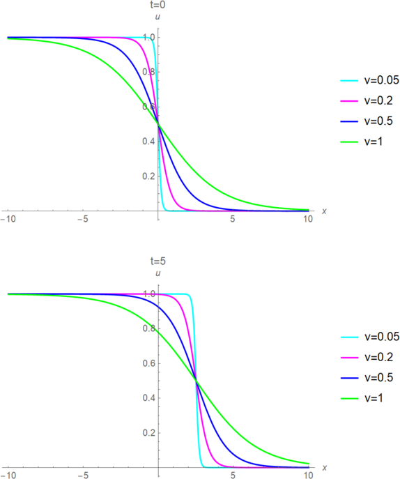
(ii) Regarding the one-dimensional viscous Burgers equation

prove that an analytical solution can be obtained by means of the Tanh Method [⁠2⁠, ⁠3⁠, ⁠5⁠] as

M. A. Xenos and A. C. Felias (Department of Mathematics, University of Ioannina, Greece)

Solution by the proposers

Notice that, for $\nabla p=\mathbf{F}=\mathbf{0}$, equation (⁠20⁠) becomes

Since, for an incompressible fluid, $\rho$ is a nonzero constant, one can divide both sides of equation (⁠23⁠) by $\rho$ and thus obtain equation (⁠21⁠). Now consider the motion of a one-dimensional viscous fluid with fluid velocity $u$ along the $x$-axis as time passes, $u=u(x,t)$. In this case, equation (⁠21⁠) transforms into equation (⁠22⁠