On the dynamics of dilute gases

1 A statistical approach to dilute gas dynamics

1.1 The physical model: A dilute gas of hard spheres

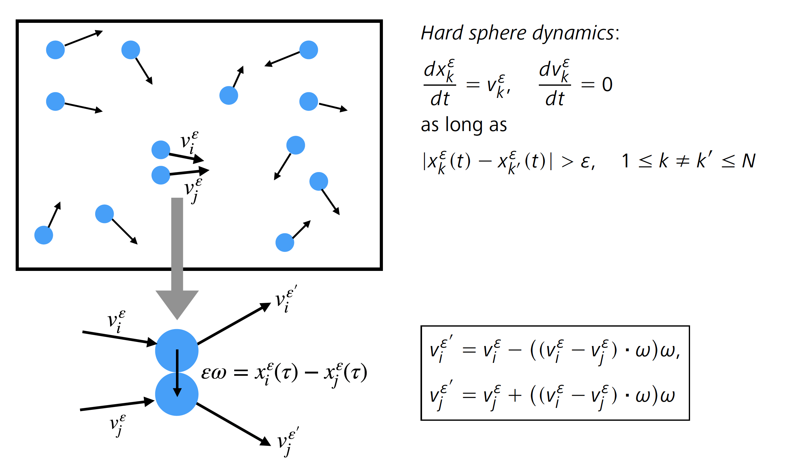
Although at the time Boltzmann published his famous paper [⁠8⁠ L. Boltzmann, Weitere Studien über das Wärmegleichgewicht unter Gasmolecülen. Wien. Ber. 66, 275–370 (1872) ] the atomic theory was still rejected by some scientists, it was already well established that matter is composed of atoms, which are the elementary constituents of all solids, liquids and gases. The particularity of gases is that the volume occupied by their atoms is negligible as compared to the total volume occupied by the gas, and there are therefore very few constraints on the atoms’ geometric arrangement: they are thus very loosely bound and almost independent. Neglecting the internal structure of the atoms, their possible organization into molecules, and the effect of long-range interactions, a gas can be represented as a system formed by a large number of particles that move in a straight line and occasionally collide with each other, resulting in an almost instantaneous scattering. The simplest example of such a model consists in assuming that the particles are small identical spheres, of diameter $\varepsilon\ll 1$ and mass 1, interacting only by contact (Figure ⁠1⁠). We refer to this as a gas of hard spheres. This microscopic description of a gas is explicit, but very difficult to use in practice because the number of particles is extremely large, their size is tiny and their collisions are very sensitive to small shifts (Figure ⁠2⁠). This model is therefore not efficient for making theoretical predictions. A natural question is whether one can extract, from such a complex system, less precise but more stable models suitable for applications, such as kinetic or fluid models. This question was formalized by Hilbert at the International Congress of Mathematicians in 1900, in his sixth problem:

Boltzmann’s work on the principles of mechanics suggests the problem of developing mathematically the limiting processes, there merely indicated, which lead from the atomistic view to the laws of motion of continua.

The Boltzmann equation, mentioned by Hilbert and described in more detail below, expresses that the particle distribution evolves under the combined effect of free transport and collisions. For these two effects to be of the same order of magnitude, a simple calculation shows that, in dimension $d\geq 2$, the number of particles $N$ and their diameter $\varepsilon$ must satisfy the scaling relation $N\varepsilon^{d-1}=O(1)$, called low density scaling [⁠14⁠ H. Grad, Principles of the kinetic theory of gases. Handbuch der Physik 12, Thermodynamik der Gase, Springer, Berlin, 205–294 (1958) ]. Indeed, the regime described by the Boltzmann equation is such that the mean free path, i.e., the average distance traveled by a particle moving in a straight line between two collisions, is of order 1. Thus, a typical particle should go through a tube of volume $O(\varepsilon^{d-1})$ between two collisions, and on average, this tube should cross one of the $N-1$ other particles. Note that, in this regime, the total volume occupied by the particles at a given time is proportional to $N\varepsilon^{d}$ and is therefore negligible compared to the total volume occupied by the gas. We speak then of a dilute gas.

1.2 Three levels of averaging

Henceforth, it is assumed that the particle system evolves in the unit domain with periodic boundary conditions $\mathbb{T}^{d}=[0,1]^{d}$. We consider that the $N$ particles are identical: this is the exchangeability assumption. The state of the system can be represented by a measure in the phase space $\mathbb{T}^{d}\times\mathbb{R}^{d}$ called empirical measure,

where $\delta_{x}$ is the Dirac mass at $x=0$. This measure is completely symmetric (i.e., invariant under permutation of the indices of the particles) because of the exchangeability assumption. This first averaging is however not sufficient to obtain a robust description of the dynamics when $N$ is large, because of the instabilities mentioned in the previous section (Figure ⁠2⁠) which lead to a strong dependence of the particle trajectories on $\varepsilon$. We will therefore introduce a second averaging, with respect to the initial configurations; from a physical point of view, this averaging is natural since only fragmentary information on the initial configuration is available. We therefore assume that the initial data $(X_{N},V_{N})=(x_{i},v_{i})_{1\leq i\leq N}$ are independent random variables, identically distributed according to a distribution $f^{0}=f^{0}(x,v)$. This assumption must be slightly corrected to account for particle exclusion: $\lvert x_{i}-x_{j}\rvert>\varepsilon$ for $i\neq j$. This statistical framework is called the canonical setting. It is a simple framework allowing us to establish rigorous foundations for the kinetic theory, i.e., to characterize, in the large $N$ asymptotics, the average dynamics and more precisely the evolution equation governing the distribution $f(t,x,v)$ at time $t$ of a typical particle. In this paper, our aim is to go beyond this averaged dynamics, and to describe in a precise way the correlations that appear dynamically inside the gas. Fixing a priori the number $N$ of particles induces additional correlations, so to circumvent them, we introduce a third level of averaging by assuming that $N$ is also a random variable, and that only its average $\mu_{\varepsilon}=\varepsilon^{-(d-1)}$ is determined (according to the low density scaling). To define a system of initially independent (modulo exclusion) identically distributed hard spheres according to $f^{0}$, we introduce the grand canonical measure as follows: the probability density of finding $N$ particles of coordinates $(x_{i},v_{i})_{i\leq N}$ is given by

where the constant $\mathcal{Z}^{\varepsilon}$ is the normalization factor of the probability measure. We will assume in the following that the function $f^{0}$ is Lipschitz continuous, with a Gaussian decay in velocity. The corresponding probability and expectation will be denoted by $\mathbb{P}_{\varepsilon}$ and $\mathbb{E}_{\varepsilon}$.

1.3 A statistical approach

Once the initial random configuration $(N,(x_{i}^{\varepsilon 0},v_{i}^{\varepsilon 0})_{1\leq i\leq N})$ is chosen, the hard sphere dynamics evolves deterministically (according to the hard sphere equations shown in Figure ⁠1⁠), and we seek to understand the statistical behavior of the empirical measure

and its evolution in time.

A law of large numbers

The first step is to determine the law of large numbers, that is, the limiting distribution of a typical particle when $\mu_{\varepsilon}\to\infty$. In the case of $N$ identically distributed independent variables $(\eta_{i})_{1\leq i\leq N}$ of expectation $\mathbb{E}(\eta)$, the law of large numbers implies in particular that the mean converges in probability to the expectation:

One can easily show the following convergence in probability:

under the grand canonical measure. The difficulty is to understand whether the initial quasi-independence propagates in time so that there exists a function $f=f(t,x,v)$ such that the following convergence in probability holds:

under the grand canonical measure (⁠1.1⁠) over the initial configurations. The most important result proving this convergence was obtained by Lanford [⁠16⁠ O. E. Lanford, III, Time evolution of large classical systems. In Dynamical systems, theory and applications (Rencontres, Battelle Res. Inst., Seattle, 1974), Lecture Notes in Phys. 38, Springer, Berlin, 1–111 (1975) ]: he showed that $f$ evolves according to a deterministic equation, namely the Boltzmann equation. This result will be explained in Section ⁠2.2⁠.

A central limit theorem

The approximation (⁠1.3⁠) of the empirical measure neglects two types of errors. The first is the presence of correction terms that converge to 0 when $\mu_{\varepsilon}\to+\infty$. The second is related to the probability, which must tend to zero, of configurations for which this convergence does not occur. A classical problem in statistical physics is to quantify more precisely these errors, by studying the fluctuations, i.e., the deviations between the empirical measure and its expectation. In the case of $N$ independent and identically distributed variables $(\eta_{i})_{1\leq i\leq N}$, the central limit theorem implies that the fluctuations are of order $O(1/\sqrt{N})$, and the following convergence in law holds true:

where $\mathcal{N}(0,\operatorname{Var}(\eta))$ is the normal law of variance $\operatorname{Var}(\eta)=\mathbb{E}((\eta-\mathbb{E}(\eta))^{2})$. In particular, at this scale, we find some randomness. Investigating the same fluctuation regime for the dynamics of hard sphere gases consists in considering the fluctuation field $\zeta^{\varepsilon}_{t}$ defined by duality, namely,

where $h$ is a continuous function, and $\mathbb{E}_{\varepsilon}$ the expectation with respect to the grand canonical measure. At time $0$, one can easily show that, under the grand-canonical measure, the fluctuation field $\zeta^{\varepsilon}_{0}$ converges in the low density limit to a Gaussian field $\zeta_{0}$ with covariance

A series of recent works [⁠4⁠ T. Bodineau, I. Gallagher, L. Saint-Raymond and S. Simonella, Fluctuation theory in the Boltzmann–Grad limit. J. Stat. Phys. 180, 873–895 (2020) , ⁠6⁠ T. Bodineau, I. Gallagher, L. Saint-Raymond and S. Simonella, Statistical dynamics of a hard sphere gas: Fluctuating Boltzmann equation and large deviations, preprint, arXiv:2008.10403; to appear in Ann. Math. (2023) , ⁠7⁠ T. Bodineau, I. Gallagher, L. Saint-Raymond and S. Simonella, Long-time correlations for a hard-sphere gas at equilibrium, preprint, arXiv:2012.03813; to appear in Comm. Pure and Appl. Math. (2023) , ⁠5⁠ T. Bodineau, I. Gallagher, L. Saint-Raymond and S. Simonella, Long-time derivation at equilibrium of the fluctuating Boltzmann equation, preprint, arXiv:2201.04514 (2022) ] has allowed to characterize the fluctuation field (⁠1.4⁠) and to obtain a stochastic evolution equation governing the limit process. These results are presented in Section ⁠3.3⁠.

On large deviations

The last question generally studied in a classical probabilistic approach is that of the quantification of rare events, i.e., the estimation of the probability of observing an atypical behavior (which deviates macroscopically from the mean). For independent and identically distributed random variables, this probability is exponentially small, and it is therefore natural to study the asymptotics

The limit $I(m)$ is called the large deviation functional and can be expressed as the Legendre transform of the log-Laplace transform $\mathbb{R}\ni u\mapsto\log\mathbb{E}(\exp(u\eta))$. To generalize this statement to correlated variables in a gas of hard spheres, it is necessary to compute the log-Laplace transform of the empirical measure on deterministic trajectories, which requires extremely precise control of the dynamical correlations. Note that, at time $0$, under the grand canonical measure, one can show that, for any $\delta>0$,

where $d$ is a distance on the space of measures. The dynamical cumulant method introduced in [⁠4⁠ T. Bodineau, I. Gallagher, L. Saint-Raymond and S. Simonella, Fluctuation theory in the Boltzmann–Grad limit. J. Stat. Phys. 180, 873–895 (2020) , ⁠6⁠ T. Bodineau, I. Gallagher, L. Saint-Raymond and S. Simonella, Statistical dynamics of a hard sphere gas: Fluctuating Boltzmann equation and large deviations, preprint, arXiv:2008.10403; to appear in Ann. Math. (2023) ] is a key tool for computing the exponential moments of the hard sphere distribution, thus obtaining the dynamical equivalent of this result in short time. We give an overview of these techniques in Section ⁠3⁠.

2 Typical behavior: A law of large numbers

2.1 Boltzmann’s amazing intuition

The equation that rules the typical evolution of a gas of hard spheres was heuristically proposed by Boltzmann [⁠8⁠ L. Boltzmann, Weitere Studien über das Wärmegleichgewicht unter Gasmolecülen. Wien. Ber. 66, 275–370 (1872) ] about a century before its rigorous derivation by Lanford [⁠16⁠ O. E. Lanford, III, Time evolution of large classical systems. In Dynamical systems, theory and applications (Rencontres, Battelle Res. Inst., Seattle, 1974), Lecture Notes in Phys. 38, Springer, Berlin, 1–111 (1975) ], as the “limit” of the particle system when $\mu_{\varepsilon}\to+\infty$. Boltzmann’s revolutionary idea was to write an evolution equation for the probability density $f=f(t,x,v)$ giving the proportion of particles at position $x$ with velocity $v$ at time $t$. In the absence of collisions, and in an unbounded domain, this density $f$ would be transported along the physical trajectories $x(t)=x(0)+vt$, which means that $f(t,x,v)=f^{0}(x-vt,v)$. The challenge is to take into account the statistical effect of collisions. As long as the size of the particles is negligible, one can consider that these collisions are pointwise in both $t$ and $x$. Boltzmann proposed a quite intuitive counting:

• the number of particles of velocity $v$ increases when a particle of velocity $v^{\prime}$ collides with a particle of velocity $v^{\prime}_{1}$, and takes the velocity $v$ (Figure ⁠1⁠ and (⁠2.2⁠));

• the number of particles of velocity $v$ decreases when a particle of velocity $v$ collides with a particle of velocity $v_{1}$, and is deflected to another velocity.

The probability of these jumps in velocity is described by a transition rate, called the collision cross section. For interactions between hard spheres, it is given by $((v-v_{1})\cdot\omega)_{+}$, where $v-v_{1}$ is the relative velocity of the colliding particles, and $\omega$ is the deflection vector, uniformly distributed in the unit sphere $\mathbb{S}^{d-1}\subset\mathbb{R}^{d}$. The fundamental assumption of Boltzmann’s theory is that, in a rarefied gas, the correlations between two colliding particles must be very small. Therefore, the joint probability of having two pre-colliding particles of velocities $v$ and $v_{1}$ at position $x$ at time $t$ should be well approximated by the product $f(t,x,v)f(t,x,v_{1})$. This independence property is called the molecular chaos hypothesis. The Boltzmann equation then reads

where

with the scattering rules

being analogous to those introduced in Figure ⁠1⁠, with the important difference that $\omega$ is now a random vector chosen uniformly in the unit sphere $\mathbb{S}^{d-1}$: indeed, the relative position of the colliding particles disappeared in the limit $\varepsilon\to 0$. As a result, the Boltzmann equation is singular because it involves a product of densities at a single point $x$. Boltzmann’s idea of reducing the Hamiltonian dynamics describing atomic behavior to a kinetic equation was revolutionary and paved the way to the description of non-equilibrium phenomena by mesoscopic equations. However, the Boltzmann equation (⁠2.1⁠) was first strongly criticized because it seems to violate some fundamental physical principles. It actually predicts an irreversible evolution in time: it has a Lyapunov functional, called entropy, defined by $S(t)≔-\iint f\log f(t,x,v)\,dx\,dv$, such that $\frac{d}{dt}S(t)\geq 0$, with equality if and only if the gas is in thermodynamic equilibrium. The Boltzmann equation thus provides a quantitative formulation of the second principle of thermodynamics. But at first glance, this irreversibility seems incompatible with the fact that the dynamics of hard spheres is governed by a Hamiltonian system, i.e., a system of ordinary differential equations that is completely reversible in time. Soon after Boltzmann postulated his equation, these two different behaviors were considered, by Loschmidt, as a paradox and an obstruction to Boltzmann’s theory. A fully satisfactory mathematical explanation of this question remained elusive for almost a century, until the role of probabilities was precisely identified: the underlying dynamics is reversible, but the description that is given of this dynamics is only partial and is therefore not reversible.

2.2 Typical behavior: Lanford’s theorem

Lanford’s result [⁠16⁠ O. E. Lanford, III, Time evolution of large classical systems. In Dynamical systems, theory and applications (Rencontres, Battelle Res. Inst., Seattle, 1974), Lecture Notes in Phys. 38, Springer, Berlin, 1–111 (1975) ] shows in which sense the Boltzmann equation (⁠2.1⁠) is a good approximation of the hard sphere dynamics. It can be stated as follows (this is not exactly the original formulation; see in particular Section ⁠2.4⁠ below for comments).

The time of validity $T_{\mathrm{L}}$ of the approximation is found to be a fraction of the average time between two successive collisions for a typical particle. This time is large enough for the microscopic system to undergo a large number of collisions (of the order of $\mu_{\varepsilon}$), but (much) too small to see phenomena such as relaxation to (local) thermodynamic equilibrium, and in particular hydrodynamic regimes. Physically, we do not expect this time to be critical, in the sense that the dynamics would change in nature afterwards. In fact, in practice, Boltzmann’s equation is used in many applications (such as spacecraft reentrance calculations) without time restrictions. However, it is important to note that a time restriction might not be only technical: from a mathematical point of view, one cannot exclude that the Boltzmann equation presents singularities (typically spatial concentrations that would prevent the collision term from making sense, and that would also locally contradict the low density assumption). At present, the problem of extending Lanford’s convergence result to longer times still faces serious obstacles.

2.3 Heuristics of Lanford’s proof

Let us informally explain how the Boltzmann equation (⁠2.1⁠) can be predicted from the dynamics of the particles. The goal is to transport via the dynamics the initial grand canonical measure (⁠1.1⁠) and then to project this measure at time $t$ onto the 1-particle phase space. We thus define by duality the density $F_{1}^{\varepsilon}(t,x,v)$ of a typical particle with respect to a test function $h$ by

Theorem ⁠2.1⁠ states that $F_{1}^{\varepsilon}$ converges to the solution to the Boltzmann equation $f$ in the low density limit. So let $h$ be a regular and bounded function on ${\mathbb{T}}^{d}\times{\mathbb{R}}^{d}$ and consider the evolution of the empirical measure during a short time interval $[t,t+\delta]$. Separating the different contributions according to the number of collisions, we can write

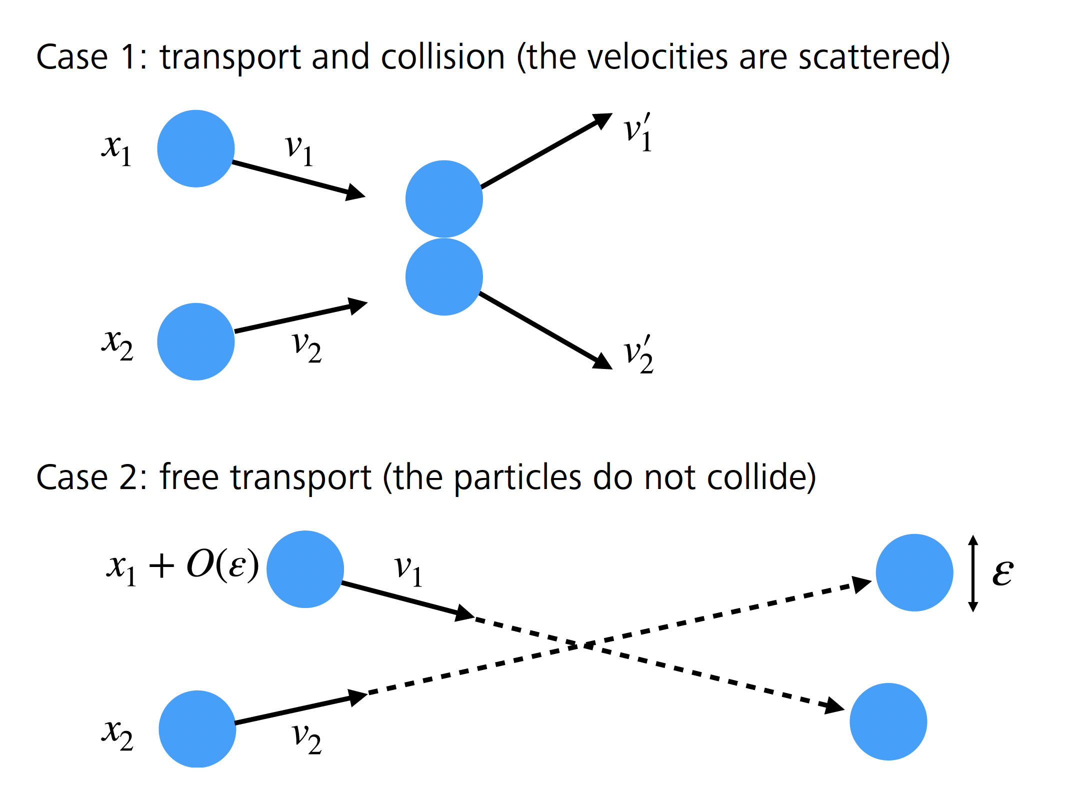
To simplify, $z^{\varepsilon}_{i}(t)$ denotes the coordinates $(x^{\varepsilon}_{i}(t),v^{\varepsilon}_{i}(t))$ of the $i$-th particle at time $t$. Since the left-hand side of (⁠2.4⁠) formally converges when $\delta\to 0$ to the time derivative of $\mathbb{E}_{\varepsilon}[\langle\pi^{\varepsilon}_{t},h\rangle]$, we will analyze the limit $\delta\to 0$ of the first two terms in the right-hand side of (⁠2.4⁠), which should lead to a transport term and a collision term as in (⁠2.1⁠). We will also explain why the remainder terms, involving two or more collisions in the short time interval $\delta$, tend to 0 with $\delta$ (showing that they are of order $\delta$). Since the particles move in a straight line and at constant speed in the absence of collisions, if the distribution $F_{1}^{\varepsilon}$ is sufficiently regular, the definition (⁠2.3⁠) of $F_{1}^{\varepsilon}$ formally implies that, when $\delta$ tends to 0, the first term in the right-hand side of (⁠2.4⁠) is asymptotically equal to

The transport term in (⁠2.1⁠) is thus well obtained in the limit. Let us now consider the second term in the right-hand side of (⁠2.4⁠). Two particles of configurations $(x_{1},v_{1})$ and $(x_{2},v_{2})$ at time $t$ collide at a later time $\tau\leq t+\delta$ if there exists $\omega\in{\mathbb{S}}^{d-1}$ such that

This implies that their relative position must belong to a tube of length $\delta\lvert v_{1}-v_{2}\rvert$ and width $\varepsilon$ oriented in the $v_{1}-v_{2}$ direction. The Lebesgue measure of this set is of the order $\delta\varepsilon^{d-1}\lvert v_{2}-v_{1}\rvert=O(\delta\varepsilon^{d-1})$ (neglecting large velocities). More generally, a sequence of $k-1$ collisions between $k$ particles imposes $k-1$ constraints of the previous form, and this event can be shown to have probability less than $(\delta\varepsilon^{d-1})^{k-1}=(\delta\mu_{\varepsilon}^{-1})^{k-1}$ (again neglecting large velocities). Since there are, on average, $\mu_{\varepsilon}^{k}$ ways to choose these $k$ colliding particles, we deduce that the occurrence of $k-1$ collisions in (⁠2.4⁠) has a probability of order $\delta^{k-1}\mu_{\varepsilon}$. This explains why the probability of having $k\geq 3$ colliding particles can be estimated by $O(\delta^{2})$ and thus can be neglected in (⁠2.4⁠). It remains to examine more closely the collision term involving two particles in (⁠2.4⁠), in order to obtain the collision operator $C(f,f)$ of the Boltzmann equation (⁠2.1⁠). This term involves the two-particle correlation function $F_{2}^{\varepsilon}$. For any $k\geq 1$, we define

where $i_{1},\dots,i_{k}$ are all distinct and $Z_{k}=(x_{i},v_{i})_{1\leq i\leq k}$. We can then show that, in the limit $\delta\to 0$,

where

The key step in closing the equation is the molecular chaos assumption postulated by Boltzmann, which states that the pre-collisional particles remain independently distributed at all times so that, with the convention (⁠2.5⁠) fixing the sign of $\omega$, we have

When the diameter $\varepsilon$ of the spheres tends to 0, the coordinates $x_{1}$ and $x_{2}$ coincide and the scattering parameter $\omega$ becomes a random parameter. Assuming that $F_{1}^{\varepsilon}$ converges, its limit must satisfy the Boltzmann equation (⁠2.1⁠). Establishing the factorization (⁠2.8⁠) rigorously uses a different strategy, elaborated by Lanford [⁠16⁠ O. E. Lanford, III, Time evolution of large classical systems. In Dynamical systems, theory and applications (Rencontres, Battelle Res. Inst., Seattle, 1974), Lecture Notes in Phys. 38, Springer, Berlin, 1–111 (1975) ], then completed and improved over the years: see the monographs [⁠25⁠ H. Spohn, Large scale dynamics of interacting particles. Texts and Monographs in Physics, Springer, Berlin (2012) , ⁠11⁠ C. Cercignani, R. Illner and M. Pulvirenti, The mathematical theory of dilute gases. Applied Mathematical Sciences 106, Springer, New York (1994) , ⁠10⁠ C. Cercignani, V. I. Gerasimenko and D. Y. Petrina, Many-particle dynamics and kinetic equations. Mathematics and its Applications 420, Kluwer Academic Publishers Group, Dordrecht (1997) ]. In the last few years, several quantitative convergence results have been established, and the proofs have been extended to the case of somewhat more general domains, potentials with compact support, or with super-exponential decay at infinity: see [⁠1⁠ N. Ayi, From Newton’s law to the linear Boltzmann equation without cut-off. Comm. Math. Phys. 350, 1219–1274 (2017) , ⁠12⁠ T. Dolmaire, About Lanford’s theorem in the half-space with specular reflection. Kinet. Relat. Models 16, 207–268 (2023) , ⁠13⁠ I. Gallagher, L. Saint-Raymond and B. Texier, From Newton to Boltzmann: Hard spheres and short-range potentials. Zurich Lectures in Advanced Mathematics, EMS, Zürich (2013) , ⁠17⁠ C. Le Bihan, Boltzmann–Grad limit of a hard sphere system in a box with isotropic boundary conditions. Discrete Contin. Dyn. Syst. 42, 1903–1932 (2022) , ⁠21⁠ M. Pulvirenti, C. Saffirio and S. Simonella, On the validity of the Boltzmann equation for short range potentials. Rev. Math. Phys. 26, Article ID 1450001 (2014) , ⁠22⁠ M. Pulvirenti and S. Simonella, The Boltzmann–Grad limit of a hard sphere system: Analysis of the correlation error. Invent. Math. 207, 1135–1237 (2017) ].

2.4 On the irreversibility

In this section, we will show that the answer to the irreversibility paradox lies in the molecular chaos hypothesis (⁠2.8⁠), which is valid only for specific configurations.

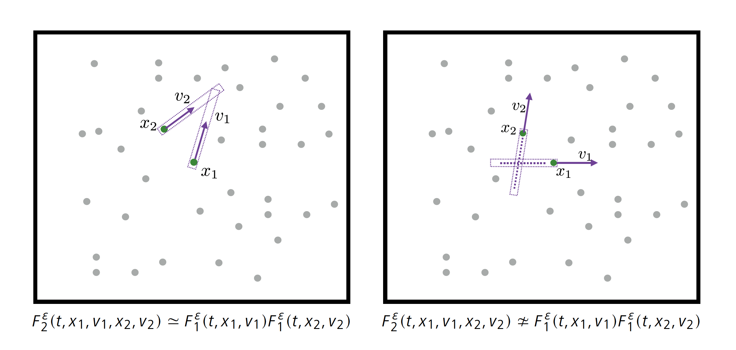
In fact, the notion of convergence that appears in the statement of Theorem ⁠2.1⁠ differs from the one used in Lanford’s proof: Theorem ⁠2.1⁠ states the convergence of the $\langle\pi^{\varepsilon}_{t},h\rangle$ observables, i.e., the convergence in the sense of measures, since the test function $h$ must be continuous. This convergence is rather weak and is not sufficient to ensure the stability of the collision term in the Boltzmann equation because this term involves traces. In the proof of Lanford’s theorem, we consider all $k$-particle correlation functions $F_{k}^{\varepsilon}$ defined by (⁠2.6⁠) and show that, when $\mu_{\varepsilon}\to\infty$, each of these correlation functions converges uniformly outside a set $\mathcal{B}_{k}^{\varepsilon}$ of negligible measure. Thus, the proof uses a much stronger notion of convergence than that stated in Theorem ⁠2.1⁠. Moreover, the set $\mathcal{B}_{k}^{\varepsilon}$ of bad microscopic configurations $(t,Z_{k})$ (on which $F^{\varepsilon}_{k}$ does not converge) is somehow transverse to the set of pre-collisional configurations (as can be seen in Figure ⁠3⁠; two particles in $\mathcal{B}_{2}^{\varepsilon}$ tend to move away from each other so that they are unlikely to collide). The convergence defect is therefore not an obstacle to taking bounds in the collision term (correlation functions are only evaluated there in pre-collisional configurations). However, these singular sets $\mathcal{B}_{k}^{\varepsilon}$ encode important information about the dynamical correlations: by neglecting them, it is no longer possible to go back in time and reconstruct the backward dynamics. Thus, by discarding the microscopic information encoded in $\mathcal{B}_{k}^{\varepsilon}$, one can only obtain an irreversible kinetic picture that is far from describing the full microscopic dynamics.

3 Fluctuations and large deviations

3.1 Corrections to the chaos assumption

Returning to equation (⁠2.7⁠) on $F_{1}^{\varepsilon}$, we can see that, apart from the small spatial shifts of the collision term, the deviations of the Boltzmann dynamics are due to the factorization defect $F_{2}^{\varepsilon}-F_{1}^{\varepsilon}\otimes\nobreak F_{1}^{\varepsilon}$, a geometric interpretation of which is given below.

Let us first describe the geometric representation of $F_{1}^{\varepsilon}$. We look at the history of particle $1^{\star}$ located at position $x_{1^{\star}}$ with velocity $v_{1^{\star}}$ at time $t$, in order to characterize all initial configurations that contribute to $F_{1}^{\varepsilon}(t,x_{1^{\star}},v_{1^{\star}})$. The particle $1^{\star}$ performs a uniform rectilinear motion $x_{1^{\star}}(t^{\prime})=x_{1^{\star}}-v_{1^{\star}}(t-t^{\prime})$ until it collides with another particle, called particle $1$, at a time $t_{1}<t$. This collision can be of two types: either a physical collision (with deflection), or a mathematical artifact arising from the loss term in equation (⁠2.7⁠) (the particles touch but are not deflected). From then on, to understand the history of particle $1^{\star}$, we need to trace the history of both particles $1^{\star}$ and $1$ before time $t_{1}$. From time $t_{1}$ on, both particles perform uniform rectilinear motions until one of them collides with a new particle $2$ at time $t_{2}<t_{1}$, and so on, until time 0. Note that, between the times of collision with new particles, the particles can collide with each other: this will be called recollision. The history of the particle $1^{\star}$ can be encoded using a rooted tree $a$ whose vertices correspond to the different collisions that took place in the history of $1^{\star}$ and are indexed by the parameters of these collisions. An example is shown in Figure ⁠4⁠. The root of the tree $a$ is indexed by $1^{\star}$. If $n$ is the total number of collisions, and $0<t_{n}<\dots<t_{1}<t$ are the times of the collisions, one can order the particles so that, at time $t_{i}$, $1\leq i\leq n$, the collision occurs between the $i$-th particle and the $j$-th particle, where $j\in\{1^{\star},1,\dots,i-1\}$ (necessarily, $j=1^{\star}$ at time $t_{1}$). Then the branching of the tree $a$ associated with the $i$-th collision is indexed by the relation $a_{i}=j$, where $j\in\{1^{\star},1,\dots,i-1\}$, together with the collision parameters $(t_{i},v_{i},\omega_{i})_{1\leq i\leq n}$, where $\omega_{i}$ is the deflection vector. The tensor product $F_{1}^{\varepsilon}\otimes F_{1}^{\varepsilon}$ is then described by two independent collision trees, with roots $1^{\star}$ and $2^{\star}$, and respectively $n_{1}$ and $n_{2}$ branches.

Now consider the second-order correlation function: $F_{2}^{\varepsilon}$ can be described by a collision graph constructed from two collision trees with roots $1^{\star}$ and $2^{\star}$, and $n_{1}+n_{2}$ branches. The main difference with $F_{1}^{\varepsilon}\otimes F_{1}^{\varepsilon}$ is that the particles in the $1^{\star}$ and $2^{\star}$ trees may interact. We can thus decompose the trees constituting $F_{2}^{\varepsilon}$ into two categories: those such that there is at least one collision involving a particle from each tree (such a recollision will be called external), and the others (Figure ⁠5⁠).

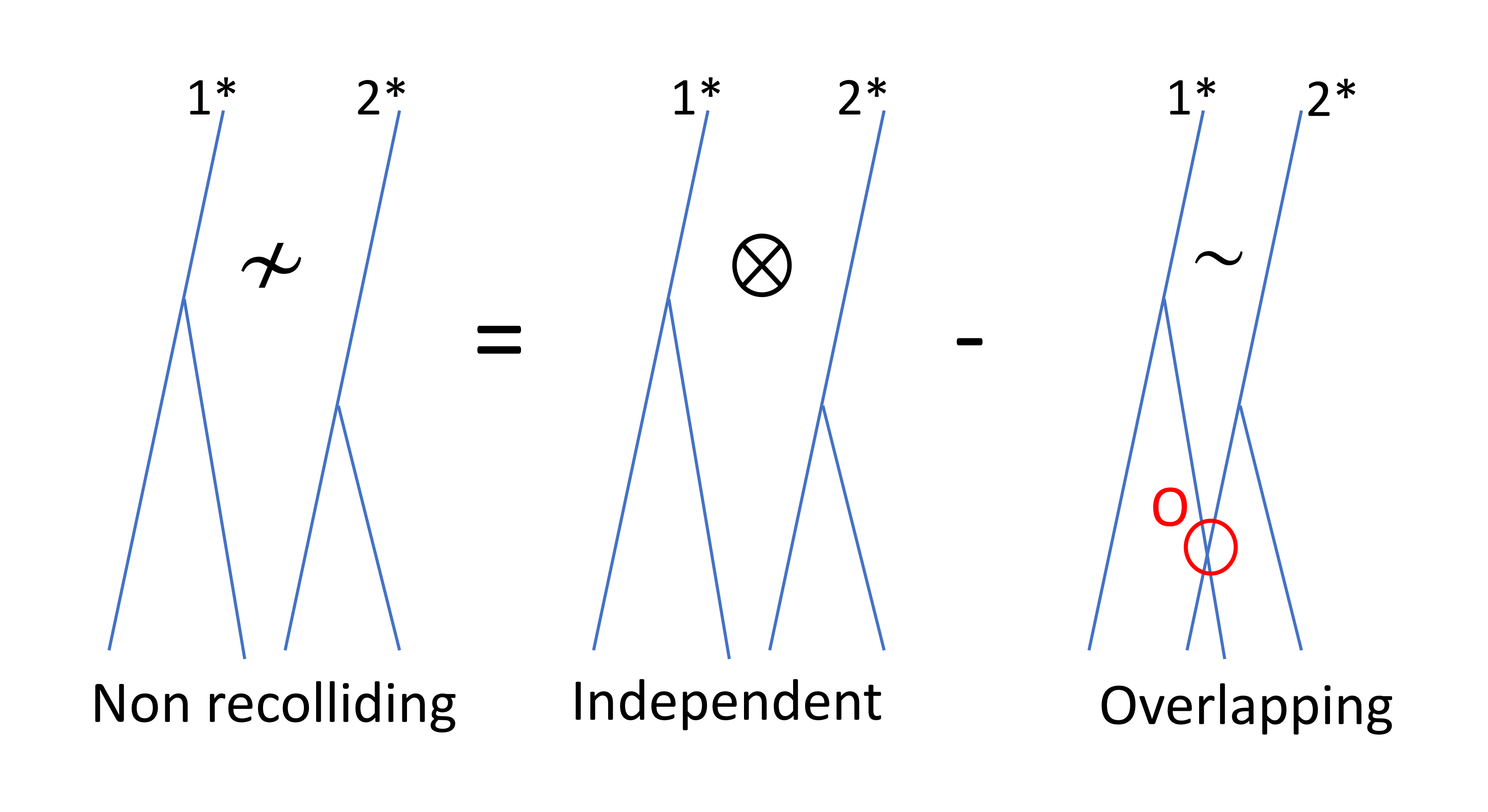
Note, however, that two collision-free trees do not correspond to independent trees, precisely because of the dynamical exclusion condition. This exclusion condition can itself be decomposed as $\mathbf{1}_{1^{\star}\not\sim 2^{\star}}=1-\mathbf{1}_{1^{\star}\sim 2^{\star}}$ (Figure ⁠6⁠), where $\mathbf{1}_{1^{\star}\sim 2^{\star}}$ means that there is an overlap at some point between a particle from the $1^{\star}$ tree and a particle from the $2^{\star}$ tree. This decomposition is a pure mathematical artifact, and the $1^{\star}\sim 2^{\star}$ overlap condition does not affect the dynamics (the overlapping particles are not deflected).

Let us now define the second-order rescaled cumulant

The previous discussion indicates that this cumulant is represented by trees that are coupled by external collisions or overlaps (Figure ⁠7⁠). In view of definition (⁠3.1⁠) and the discussion in Section ⁠2.3⁠ giving an $O(t/\mu_{\varepsilon})$ estimate of the Lebesgue measure of configurations giving rise to a collision, one can expect $f_{2}^{\varepsilon}$ to be uniformly bounded in $L^{1}$ and therefore to have a limit $f_{2}$ in the sense of the measures. One can prove in addition that $f_{2}$ corresponds to trees with exactly one external recollision or overlap on $[0,t]$: any other interaction between the trees gives rise to additional smallness and is therefore negligible.

3.2 The cumulant generating function

For a Gaussian process, the first two correlation functions $F_{1}^{\varepsilon}$ and $F_{2}^{\varepsilon}$ determine completely all other $k$-particle correlation functions $F_{k}^{\varepsilon}$, but in general, part of the information is encoded in the cumulants of higher order ($k\geq 3$)

where $\mathcal{P}^{\ell}_{k}$ is the set of partitions of $\{1,\dots,k\}$ into $\ell$ parts with $\sigma=\{\sigma_{1},\dots,\sigma_{\ell}\}$, $\lvert\sigma_{i}\rvert$ being the cardinality of the set $\sigma_{i}$ and $Z_{\sigma_{i}}=(z_{j})_{j\in\sigma_{i}}$. Each cumulant encodes finer and finer correlations. Contrary to the correlation functions $(F_{k}^{\varepsilon})$, the cumulants $(f_{k}^{\varepsilon})$ do not duplicate the information which is already encoded at lower orders. From a geometric point of view, we can extend the analysis of the previous section and show that the cumulant $f_{k}^{\varepsilon}$ of order $k$ can be represented by $k$ trees that are completely connected either by external collisions, or by overlaps (Figure ⁠8⁠). These dynamical correlations can be classified by a signed graph with $k$ vertices representing the different trees, coding tree collisions (the corresponding edges take a + sign) and overlaps (the corresponding edges take a $-$ sign). We can then systematically extract a minimally connected graph $T$ by identifying $k-1$ “aggregations” of tree collisions or overlaps. We then expect $f_{k}^{\varepsilon}$ to decompose into a sum of $2^{k-1}k^{k-2}$ terms, where the factor $k^{k-2}$ is the number of trees with $k$ numbered vertices (from Cayley’s formula). For each given signed minimally connected graph, the collision/overlap conditions correspond to $k-1$ independent constraints on the configuration $z_{1^{\star}},\dots,z_{k^{\star}}$ at time $t$. Therefore, neglecting the issue of large velocities, this contribution to the cumulant $f_{k}^{\varepsilon}$ has a Lebesgue measure of size $O((t/\mu_{\varepsilon})^{k-1})$, and we derive the estimate

A geometric argument similar to the one developed in Lanford’s proof and recalled in the analysis of the second-order cumulant above shows that $f_{k}^{\varepsilon}$ converges to a limiting cumulant $f_{k}$ and that only graphs with exactly $k-1$ external collisions or overlaps (and no cycles) contribute in the limit. Note further that a classical and rather simple calculation (based on the series expansions of the exponential and logarithm) shows that the cumulants are nothing but the coefficients of the series expansion of the exponential moment:

The quantity $\mathcal{I}^{\varepsilon}_{t}(h)$ is called the cumulant generating function. Estimate (⁠3.2⁠) provides the analyticity of $\mathcal{I}^{\varepsilon}_{t}(h)$ in short time as a function of $e^{h}$, and this uniformly with respect to $\varepsilon$ (sufficiently small). The limit $\mathcal{I}_{t}$ of $\mathcal{I}^{\varepsilon}_{t}$ can then be determined as a series in terms of the limiting cumulants $f_{k}$,

In a suitable functional setting [⁠5⁠ T. Bodineau, I. Gallagher, L. Saint-Raymond and S. Simonella, Long-time derivation at equilibrium of the fluctuating Boltzmann equation, preprint, arXiv:2201.04514 (2022) ], it can be shown that this functional satisfies a Hamilton–Jacobi equation

with initial condition $\mathcal{I}(0,h)=\int dz\,f^{0}(e^{h}-1)$ and Hamiltonian $\mathcal{H}$ given by

where $\Delta h(z_{1},z_{2},\omega)=h(z^{\prime}_{1})+h(z^{\prime}_{2})-h(z_{1})-h(z_{2})$. We use here notation (⁠2.2⁠) for the pre-collisional velocities and the definition

The successive derivatives of this functional being precisely the limit cumulants $f_{k}$, the successive derivatives of the Hamilton–Jacobi equation provide the evolution equations of these cumulants: for example, differentiating this equation once produces the Boltzmann equation, differentiating it twice produces the equation of the covariance described in the next paragraph.

3.3 Fluctuations

The control of the cumulant generating function allows in particular to obtain the convergence of the fluctuation field defined in (⁠1.4⁠) and thus to analyze the dynamical fluctuations over a time $T^{\star}$ of the same order of magnitude as the convergence time $T_{L}$ of Theorem ⁠2.1⁠.