
1 Introduction
The rigorous derivation of the evolution equations of classical fluid mechanics from the large-scale description of the conserved quantities in Newtonian particle systems is a long-standing problem in mathematical physics. More precisely, we are referring to the area of statistical mechanics dedicated to understanding the emergence of evolution laws from the kinetic description of the underlying system of particles. To attack this problem, we can assume that the motion of particles is random. We introduce two scales: a macroscopic scale, where the systems’ thermodynamical quantities, such as, e.g., density, pressure, temperature, etc. (denote them by ) are analyzed. The other one, the microscopic scale, is the scale at which the particles of the system are analyzed as a whole. As a possible scenario, one can be interested in understanding the physical evolution of a gas confined to a finite volume. The number of molecules is of the order of Avogadro’s number; therefore, one cannot give a precise description of the microscopic state of the system; rather, the goal is to describe the macroscopic behavior from the random movement of the molecules.
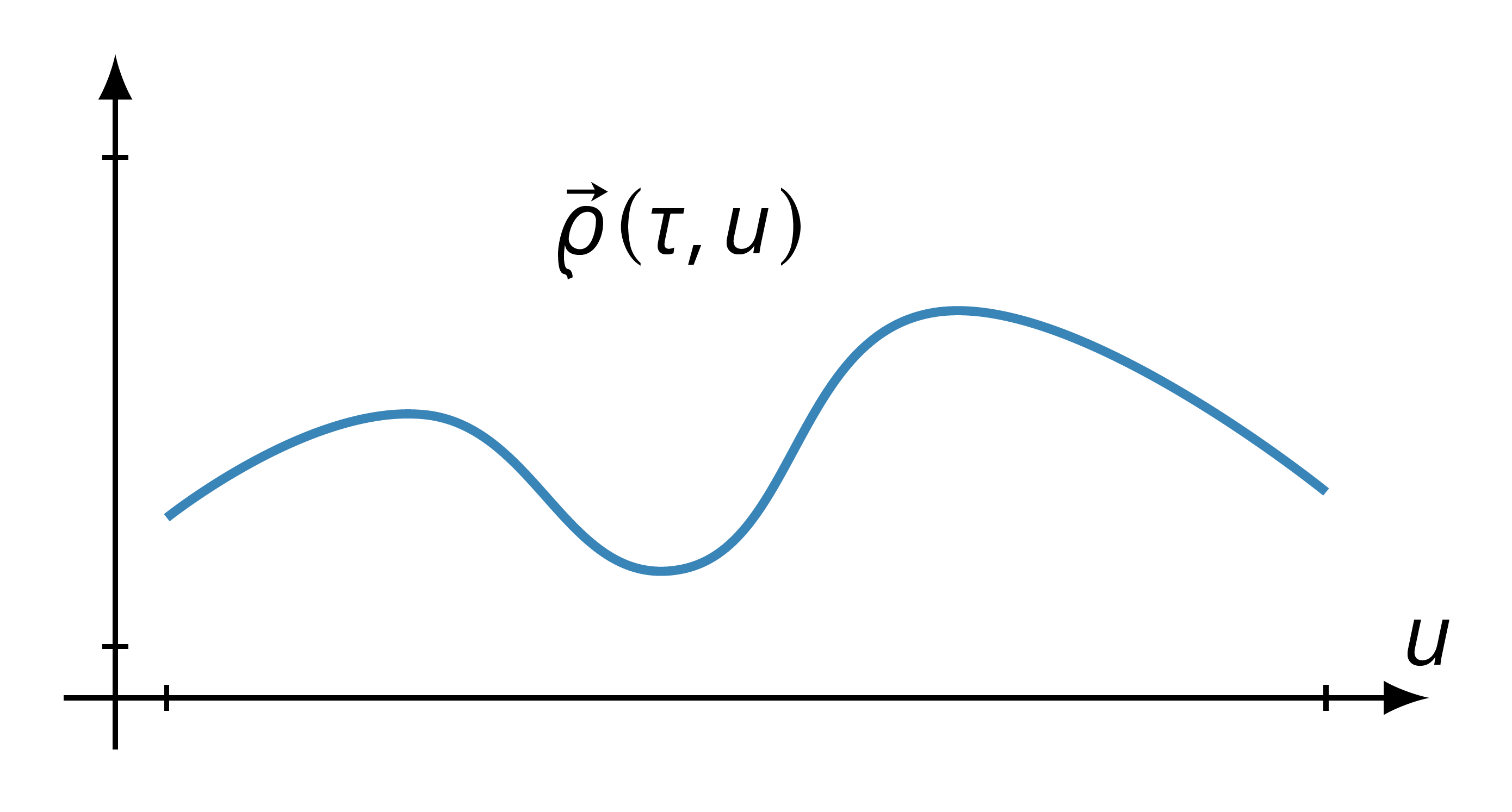
Understanding the connection between macro/micro-spaces is one of the goals in statistical mechanics. According to one of the creators of this area, Ludwig Boltzmann, first we should determine the stationary states of the system under investigation (denote them by ), and then we should characterize these states in terms of the thermodynamical quantities of interest , resulting in . Finally, we can analyze the evolution of the system out of equilibrium. To formalize this problem from the mathematical point of view, consider a macroscopic space and fix an arbitrary point and a small neighborhood around it, in such a way that it is macroscopically small, yet big enough to contain infinitely many molecules. Due to the strong interaction between molecules, we can assume that the system is locally in equilibrium so that its state at the point should be close to . Observe that this local equilibrium is characterized by the thermodynamical quantities that now depend on the position . We let time evolve, and we assume that the local equilibrium persists at a longer time. Later on, we stop the system at some time , and now the local equilibrium will be given in terms of , depending both on time and space, i.e., the state of the system should be close to . The function should then evolve according to some PDE, the so-called hydrodynamic equation.
As mentioned above, treating this problem from the mathematical point of view is challenging, and some simplifying assumptions are usually introduced. A possible approach is to consider that the dynamics of particles is random, which leads to the commonly known stochastic interacting particle systems (SIPS), which are random systems typically used in statistical mechanics to attack this sort of problems. Back in the 1970s, these systems were introduced in the mathematics community by Spitzer in [50 F. Spitzer, Interaction of Markov processes. Advances in Math. 5, 246–290 (1970) (1970) ], but were already known to physicists and biophysicists since the seminal article of MacDonald, Gibbs and Pipkin [47 C. MacDonald, J. Gibbs and A. Pipkin, Kinetics of biopolymerization on nucleic acid templates. Biopolymer 6, 1–25 (1968) ]. The dynamics of these systems conserves a certain number of quantities. At the micro-level one assumes that each molecule behaves as a continuous-time random walk evolving in a proper discretization of the macroscopic space ; this allows for a probabilistic analysis of the discrete system. For details on the formal definition of SIPS, we refer to the seminal book of Liggett [46 T. M. Liggett, Interacting particle systems. Grundlehren Math. Wiss. 276, Springer, New York (1985) ]. The obtained evolution of molecules is Markovian, i.e., their future evolution conditioned to their past depends only on the knowledge of the present. We can discretize the volume according to a scaling parameter . At each site of the discrete set, we can place randomly a certain number of particles and repeat this independently of all the other sites. In this way, we have just fixed the initial state of the system. Each one of these particles waits an exponentially distributed time, after which one of them jumps to some other site if the dynamical rules allow for it. Once the dynamics is fixed, according to Boltzmann, one should find the stationary measures and characterize them in terms of the relevant thermodynamical quantities.
The goal, in the hydrodynamic limit, is to obtain the PDEs that govern the space-time evolution of each conserved quantity of the system studied [45 C. Kipnis and C. Landim, Scaling limits of interacting particle systems. Grundlehren Math. Wiss. 320, Springer, Berlin (1999) , 51 H. Spohn, Large scale dynamics of interacting particles. Texts and Monographs in Physics, Springer, Berlin (1991). ]. The macroscopic and microscopic spaces will be connected by means of the scaling parameter so that the typical distance between particles is of order . At the end, will be taken to . To observe a non-trivial macroscopic impact of the particles’ motion, one has to look at the system on a longer time scale , which depends on the scaling parameter and on the dynamical rules. If the dynamical rules allow a strong long-range interaction, then the time needed for a macroscopic effect is shorter compared to a dynamics that allows very short-range interactions.
2 Hydrodynamic limit
In order to exhibit PDEs that can be obtained for some SIPS, in the next subsections, we describe the hydrodynamic limit for a system with a single conservation law, and then we discuss the case with more conservation laws.
2.1 A classical SIPS: The exclusion process
The model
One of the most classical SIPS is the exclusion process, whose dynamics can be described as follows. Recall that is the scaling parameter connecting the macroscopic space and the microscopic space . Assume that, at each site of , there can be at most one particle (the so-called exclusion rule) so that if is a configuration, then denotes the number of particles at site and at time , and . To each bond of , there is attached a Poisson process of rate one. The trajectories of Poisson processes are discontinuous, and at each site where a discontinuity occurs, we say that there is a mark of the Poisson process. Poisson processes attached to different bonds are independent. This means that particles have to wait for a random time which is exponentially distributed with mean one, and when there is a mark of the Poisson process associated to a bond , the particles at that bond exchange positions at the rate , where is a transition probability. The jump occurs if and only if the exclusion rule is obeyed; otherwise, the particles wait for another mark of one Poisson process. The number of particles in the system is fixed by its initial state, and since this dynamics only exchanges particles along the microscopic space, the density is a conserved quantity.
The state space is , and when jumps are allowed only to nearest neighbors, the process is said to be simple. First, we explain phenomena observed in the case of nearest-neighbor jumps, and then we treat the extension to the long-jumps case. To that end, for now, we assume that and , where and . If and , we obtain the extensively studied symmetric simple exclusion process (SSEP); if , but , we get the asymmetric simple exclusion process (ASEP); and if and , we get the weakly asymmetric simple exclusion process (WASEP). Observe that the parameter rules the strength of the asymmetry. The infinitesimal generator of the described process is given on and by
where and is the configuration obtained from by swapping the occupation variables at and . We can think of as a differential operator that, when testing functions defined on the state space of the process, gives a weight which is the product between the jump rate and the difference between the values of the function at the configurations after and before the jump. This operator corresponds to the time derivative of the semigroup of the process via the formula
Now let us speed the system in the time scale , where will be chosen ahead in order to see a non-trivial macroscopic evolution. The system conserves a single quantity: the number of particles . Next, we should obtain the stationary measures of this process and parametrize them by a constant density . By this, we mean that if we denote by a stationary measure of the process, then if the initial process has distribution , i.e., the law of is given by , then at any time , the same holds, i.e., the law of is given again by . For the exclusion processes defined above, the space-time invariant measures are Bernoulli product measures of parameter :
and in fact, these measures are reversible for some choices of . The latter means that the adjoint generator in the Hilbert space coincides with .
Hydrodynamic limit of exclusion processes
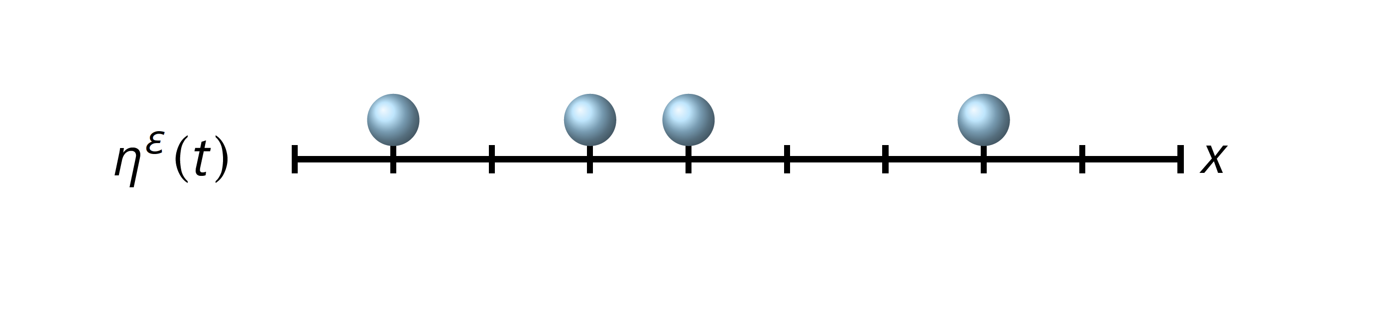
The empirical measure associated to the number of particles is given on by
where is a Dirac mass at . Observe that, for a given configuration , the measure gives weight to each particle. We define the process of empirical measures as .
The rigorous statement of the hydrodynamic limit is that, given a measurable profile , if the process starts from a probability measure for which a Law of Large Numbers (LLN) for holds, i.e.,
then the same holds at any time , i.e.,
where is the solution (in some sense) of the hydrodynamic equation. Observe that the assumption above says that the random measure converges weakly, as , to the deterministic measure . This means that, for any given continuous function , one has
But we still need to say in which sense the convergence holds because the left-hand side of the last display is still random. We will assume that the convergence is in probability with respect to , i.e., for any , one has
And this will be a restriction on the set of initial measures for which the result will be derived.
Hydrodynamic equations
To provide an intuition of which equations can be derived from SIPS, we give now a heuristic argument for the exclusion processes defined above. Recall that, for these processes, the invariant measures are the Bernoulli product with marginals given in (1). Consider the discrete profile
From Kolmogorov’s equation, we have that , and a simple computation shows that
where denotes the instantaneous current at the bond . Assume now that the process at hand is the SSEP. Then
Since is the gradient of , we get , where denotes the discrete Laplacian. Here the expectation is with respect to the Bernoulli product measure given in (1), but with a parameter given by . Now, if we assume that for all , then the evolution of the density is given by the heat equation . Of course, we worked under the local equilibrium assumption made above, but this heuristic argument can be made rigorous by certain methods and for many different models.
For the exclusion process introduced above, we can get the following hydrodynamic equations [19 A. De Masi, E. Presutti and E. Scacciatelli, The weakly asymmetric simple exclusion process. Ann. Inst. H. Poincaré Probab. Statist. 25, 1–38 (1989) , 43 L. Jensen and H.-T. Yau, Hydrodynamical scaling limits of simple exclusion models. In Probability theory and applications (Princeton, NJ, 1996), IAS/Park City Math. Ser. 6, Amer. Math. Soc., Providence, 167–225 (1999) , 45 C. Kipnis and C. Landim, Scaling limits of interacting particle systems. Grundlehren Math. Wiss. 320, Springer, Berlin (1999) ]:
a. SSEP with , the heat equation
b. WASEP with , the viscous Burgers equation
c. ASEP with , the inviscid Burgers equation
For symmetric , i.e., such that for all , allowing long jumps with infinite variance, e.g.,
we obtain a fractional heat equation, namely,
for ; see [42 M. Jara, Hydrodynamic limit of particle systems with long jumps, preprint, arXiv:0805.1326 (2008) ]. Note that the infinite variance case corresponds to since, in this range, . When is asymmetric, one can obtain an integro-PDE [49 S. Sethuraman and D. Shahar, Hydrodynamic limits for long-range asymmetric interacting particle systems. Electron. J. Probab. 23, Paper No. 130 (2018) ]. All these equations can be supplemented with several types of boundary conditions by superposing the dynamics described above with another one, for example, by
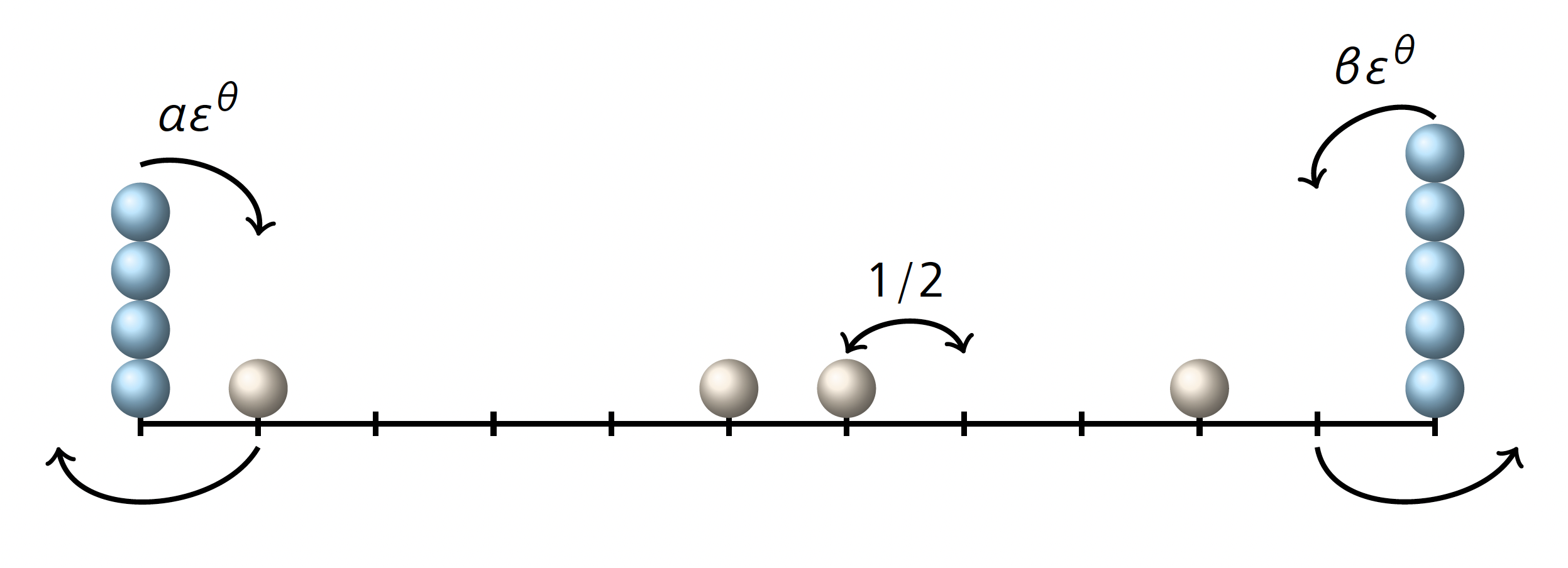
1. Considering the exclusion process evolving on the lattice
and adding at the boundary points and a dynamics that injects particles (at rate and at the left and right reservoir respectively) or removes particles (at rate and at the left and right reservoir respectively) in the system.
The parameters satisfy and . Note that the conservation law is violated in this case, but inside the system, it still holds.
2. Considering the exclusion process with a dynamics that blocks the passage of particles between certain regions of the microscopic space (the conservation law is maintained in this case). For instance, assume that the exchange rate of particles in a certain number of bonds is given by a transition probability , while in some other bonds, this rate is multiplied by a factor that makes it slower compared to the rate in all other bonds. In Figure 2, particles jump everywhere in , but the jump rate for bonds in or in is given by , whereas the jump rate between sites in and is given by , where now the parameters satisfy and .

Under this choice, we are creating a slow barrier at the macroscopic level, and the goal is to understand how these local microscopic defects propagate to the macroscopic level. Here we do not have a superposition of two dynamics; as in the previous case, we are just slowing down the dynamics in certain places of the microscopic space.
For recent results on 1., we refer to [3 R. Baldasso, O. Menezes, A. Neumann and R. R. Souza, Exclusion process with slow boundary. J. Stat. Phys. 167, 1112–1142 (2017) , 20 A. De Masi, E. Presutti, D. Tsagkarogiannis and M. E. Vares, Current reservoirs in the simple exclusion process. J. Stat. Phys. 144, 1151–1170 (2011) , 26 C. Franceschini, P. Gonçalves and B. Salvador, Hydrodynamical behavior for the generalized symmetric exclusion with open boundary; to appear in Math. Phys. Anal. Geom. , 22 C. Erignoux, P. Gonçalves and G. Nahum, Hydrodynamics for SSEP with non-reversible slow boundary dynamics: Part I, the critical regime and beyond. J. Stat. Phys. 181, 1433–1469 (2020) , 23 C. Erignoux, P. Gonçalves and G. Nahum, Hydrodynamics for SSEP with non-reversible slow boundary dynamics: Part II, below the critical regime. ALEA Lat. Am. J. Probab. Math. Stat. 17, 791–823 (2020) ] for the SSEP in contact with slow/fast boundary reservoirs. In that case, the heat equation is supplied with boundary conditions of Dirichlet, Robin, or Neumann type, depending on the intensity of the reservoirs’ dynamics. More precisely, we can get the heat equation (3) with the following boundary conditions:
(I) Dirichlet: , if .
(II) Robin: , if .
(III) Neumann: if . For the WASEP, one can get the viscous Burgers equation (4) with Dirichlet conditions as in (I) or with Robin boundary conditions, but in this case, the boundary conditions are nonlinear; see [14 P. Capitão and P. Gonçalves, Hydrodynamics of weakly asymmetric exclusion with slow boundary. In From particle systems to partial differential equations, Springer Proc. Math. Stat. 352, Springer, Cham, 123–148 (2021) ]. For the ASEP, the parabolic equations obtained above are replaced by hyperbolic laws with several types of boundary conditions [2 C. Bahadoran, Hydrodynamics and hydrostatics for a class of asymmetric particle systems with open boundaries. Comm. Math. Phys. 310, 1–24 (2012) , 54 L. Xu, Hydrodynamics for one-dimensional ASEP in contact with a class of reservoirs. J. Stat. Phys. 189, Paper No. 1 (2022) ].
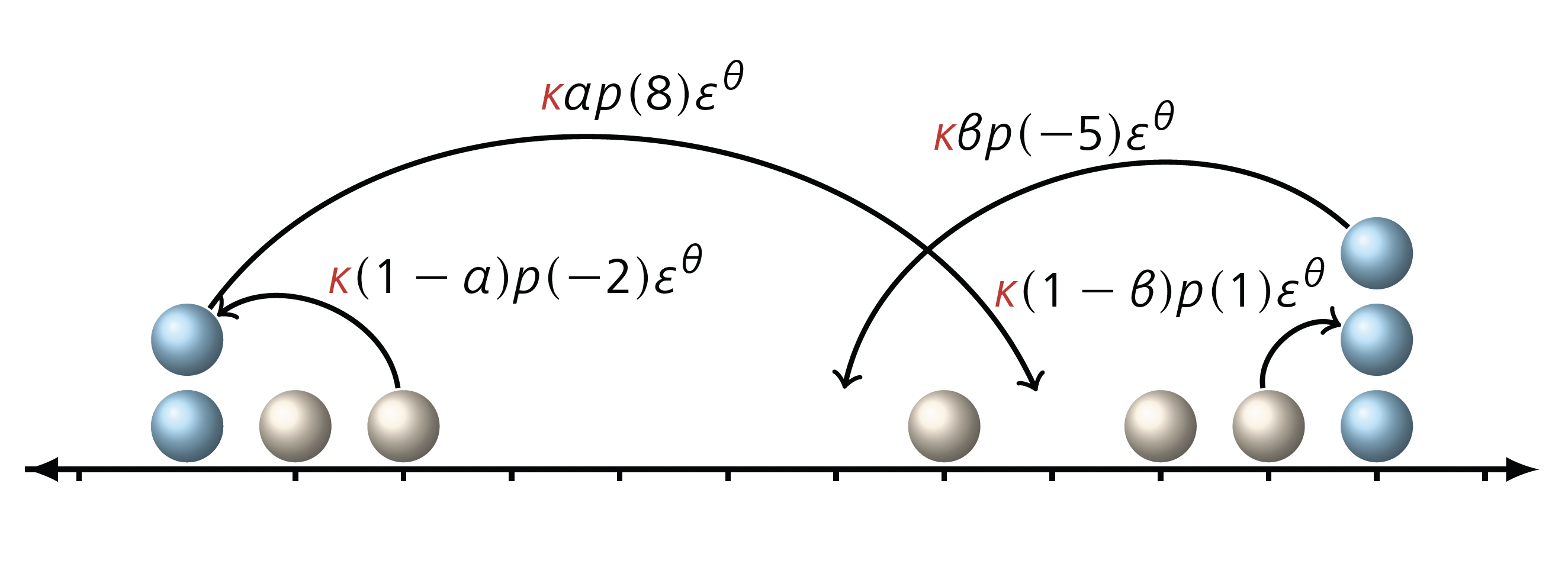
For the dynamics defined in 1., but in the case of long jumps, we refer to [9 C. Bernardin, P. Gonçalves and B. Jiménez-Oviedo, Slow to fast infinitely extended reservoirs for the symmetric exclusion process with long jumps. Markov Process. Related Fields 25, 217–274 (2019) , 10 C. Bernardin, P. Gonçalves and B. Jiménez-Oviedo, A microscopic model for a one parameter class of fractional Laplacians with Dirichlet boundary conditions. Arch. Ration. Mech. Anal. 239, 1–48 (2021) , 4 C. Bernardin, P. Cardoso, P. Gonçalves and S. Scotta, Hydrodynamic limit for a boundary driven super-diffusive symmetric exclusion, preprint, arXiv:2007.01621 (2021) ], where the authors consider the transition probability (5), superposed with a dynamics that injects and removes particles in the system and that acts everywhere in with a strength regulated again by a parameter ; see Figure 3.
Depending on whether the variance of the transition probability is finite or not and on the strength of the Glauber dynamics, the variety of results for the hydrodynamic limit is extremely rich: indeed, different operators arise at the macro-level, and the corresponding equations come equipped with several types of boundary conditions of fractional form.
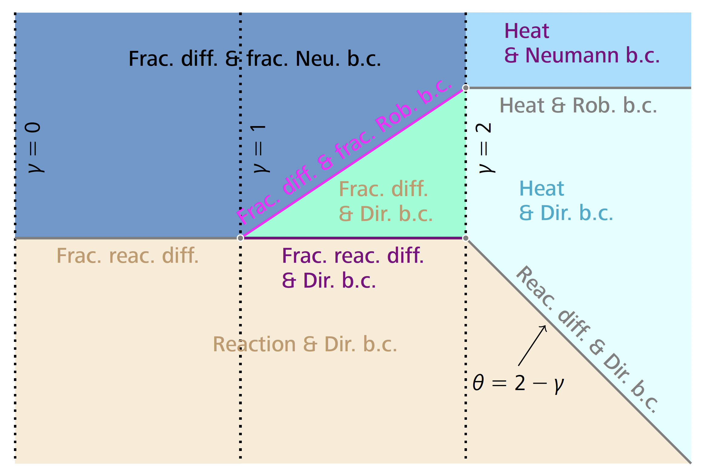
When the transition probability has finite variance, i.e., , which holds for , the hydrodynamic equation for is the heat equation with various boundary conditions. When , the variance diverges as , and to compensate for this, we have to take the time scale to obtain again the heat equation with several kinds of boundary conditions.
When , the variance is infinite and the system becomes superdiffusive. Consequently, the resulting equation is written in terms of a fractional Laplacian operator rather than the ordinary Laplacian. Since the solutions of the equation are defined on the interval , one deals, in fact, with a regional fractional Laplacian. Now the boundary conditions involve fractional derivatives. For a summary of the regimes where the boundary conditions are shown, see Figure 4.
For recent results on 2., we refer the reader to [27 T. Franco, P. Gonçalves and A. Neumann, Hydrodynamical behavior of symmetric exclusion with slow bonds. Ann. Inst. Henri Poincaré Probab. Stat. 49, 402–427 (2013) , 28 T. Franco, P. Gonçalves and A. Neumann, Phase transition of a heat equation with Robin’s boundary conditions and exclusion process. Trans. Amer. Math. Soc. 367, 6131–6158 (2015) ] for the SSEP with a slow bond on the torus
to [29 T. Franco, P. Gonçalves and G. M. Schütz, Scaling limits for the exclusion process with a slow site. Stochastic Process. Appl. 126, 800–831 (2016) ] for the SSEP with a slow site on , and to [16 P. Cardoso, P. Gonçalves and B. Jiménez-Oviedo, Hydrodynamic behavior of long-range symmetric exclusion with a slow barrier: Diffusive regime; to appear in Ann. Inst. Henri Poincaré Probab. Stat. , 17 P. Cardoso, P. Gonçalves and B. Jiménez-Oviedo, Hydrodynamic behavior of long-range symmetric exclusion with a slow barrier: Superdiffusive regime; accepted for publication in Ann. Sc. Norm. Super. Pisa Cl. Sci. (5) ] for the SSEP on with a slow barrier blocking the passage of particles.
We note that, in the case of a slow barrier, the variety of hydrodynamic limits is also very rich. When the intensity of the barrier is equal to and slows down the passage of particles between negative and positive sites on , an interesting behavior appears (contrarily to the slow bond case of [27 T. Franco, P. Gonçalves and A. Neumann, Hydrodynamical behavior of symmetric exclusion with slow bonds. Ann. Inst. Henri Poincaré Probab. Stat. 49, 402–427 (2013) ]) when :
(i) For , in [42 M. Jara, Hydrodynamic limit of particle systems with long jumps, preprint, arXiv:0805.1326 (2008) ], the author obtains the fractional heat equation.
(ii) For , the fractional Laplacian is replaced by a regional fractional Laplacian, but defined on an unbounded domain. In this case, since there are infinitely many slow bonds at the microscopic level, the impact of their slowed dynamics (which differs from the dynamics of other bonds only by a constant) is felt at the macroscopic level.
(iii) For and , one can get linear-fractional Robin boundary conditions.
(iv) For and , one can get fractional Neumann boundary conditions. Note that, while above we arrived at the heat equation or the fractional heat equation, it is possible to obtain a nonlinear version of those equations of the form , where and or , i.e., the porous medium equation and its fractional version. For details, we refer the reader to [21 R. De Paula, P. Gonçalves and A. Neumann, Energy estimates and convergence of weak solutions of the porous medium equation. Nonlinearity 34, 7872–7915 (2021) , 13 L. Bonorino, R. de Paula, P. Gonçalves and A. Neumann, Hydrodynamics of porous medium model with slow reservoirs. J. Stat. Phys. 179, 748–788 (2020) , 15 P. Cardoso, R. De Paula and P. Gonçalves, A microscopic model for the fractional porous medium equation; to appear in Nonlinearity ]. To arrive at these PDEs, one can simply start with an exclusion dynamics where the jump rate depends on the number of particles in the vicinity of the point where particles exchange positions; see [38 P. Gonçalves, C. Landim and C. Toninelli, Hydrodynamic limit for a particle system with degenerate rates. Ann. Inst. Henri Poincaré Probab. Stat. 45, 887–909 (2009) , 13 L. Bonorino, R. de Paula, P. Gonçalves and A. Neumann, Hydrodynamics of porous medium model with slow reservoirs. J. Stat. Phys. 179, 748–788 (2020) , 15 P. Cardoso, R. De Paula and P. Gonçalves, A microscopic model for the fractional porous medium equation; to appear in Nonlinearity ].
2.2 Two conservation laws
In this subsection, we review the hydrodynamic limit for two different models with more than one conservation law. The analysis of the asymptotic behavior of the relevant quantities is much more intricate than for models with just one conserved quantity, such as the exclusion process described above.
2.2.1 The ABC model
The model
The ABC model consists of a system of particles of three species , with exchanges only to neighboring sites on the torus and in the presence of a driving force, so the interaction rate depends on the type of particles involved. As in the exclusion process explained previously, at each site, there is at most one particle. The total number of particles of each species is conserved. This is a continuous-time Markov process with state space . To properly define its hydrodynamic limit, we introduced the occupation number of the species as , which acts on configurations by the rule . Its infinitesimal generator acts on functions as
Here the rates are defined by
where a configuration on the bond is exchanged to at the rate
for , with . The role of in this model is to tune the strength of the driving force. This model generalizes the one introduced in [24 M. R. Evans, Y. Kafri, H. M. Koduvely and D. Mukamel, Phase separation in one-dimensional driven diffusive systems. Phys. Rev. Lett. 80, 425–429 (1998) , 25 M. R. Evans, Y. Kafri, H. M. Koduvely and D. Mukamel, Phase separation and coarsening in one-dimensional driven diffusive systems: Local dynamics leading to long-range Hamiltonians. Phys. Rev. E (3) 58, 2764–2778 (1998) ]. The system will be considered in the diffusive time scale . We can think of this model as a two-species particle system, of species and , since the type can be easily recovered from and .
We introduce the empirical measure (defined similarly to (2)) for each one of the conserved quantities , and , i.e., for each , we define
Hydrodynamic limit of ABC
In the diffusive time scaling and for , for any , the empirical measure
converges as to the deterministic measure
where the densities solve the following system of (parabolic) equations [12 L. Bertini, N. Cancrini and G. Posta, On the dynamical behavior of the ABC model. J. Stat. Phys. 144, 1284–1307 (2011) ]:
here , and for , denotes the density of particles of type in the system. The equation for the species can easily be obtained by using the identity . In this case, the hydrodynamic limit is given by a system of coupled equations since the evolution of particles of one species is affected by the particles of the other species. One can also consider this model in contact with slow/fast reservoirs, extending the model defined above. Consider, for example, the dynamics described in Figure 5.

The rates satisfy and , and can be interpreted as density reservoirs. For this model, the hydrodynamic equation is similar to (6), and it is supplemented with boundary conditions that can be of Dirichlet type or Robin type [39 P. Gonçalves, R. Misturini and A. Occelli, Hydrodynamics for the ABC model with slow/fast boundary; to appear in Stochastic Process. Appl. ].
2.2.2 Interface models
The models
Next, we describe another collection of models with two conservation laws. These systems were introduced in [11 C. Bernardin and G. Stoltz, Anomalous diffusion for a class of systems with two conserved quantities. Nonlinearity 25, 1099–1133 (2012) ]; they consist of perturbations of Hamiltonian dynamics with a conservative noise and exhibit strong analogies with the standard chains of oscillators. The dynamics of these fluctuating interface models, denoted by , depends on an interaction potential and evolves in the state space (these variables now are continuous and unbounded). The dynamics conserves two quantities:
and in [11 C. Bernardin and G. Stoltz, Anomalous diffusion for a class of systems with two conserved quantities. Nonlinearity 25, 1099–1133 (2012) ], it is proved that these are the only conserved quantities. Here stands for the height of the interface at the site .
There are some potentials that have been explored in the literature. Below, we focus on two of them, namely, the exponential potential and the quadratic potential; see [1 R. Ahmed, C. Bernardin, P. Gonçalves and M. Simon, A microscopic derivation of coupled SPDE’s with a KPZ flavor. Ann. Inst. Henri Poincaré Probab. Stat. 58, 890–915 (2022) , 5 C. Bernardin and P. Gonçalves, Anomalous fluctuations for a perturbed Hamiltonian system with exponential interactions. Comm. Math. Phys. 325, 291–332 (2014) , 6 C. Bernardin, P. Gonçalves and M. Jara, 3/4-fractional superdiffusion in a system of harmonic oscillators perturbed by a conservative noise. Arch. Ration. Mech. Anal. 220, 505–542 (2016) , 7 C. Bernardin, P. Gonçalves and M. Jara, Weakly harmonic oscillators perturbed by a conservative noise. Ann. Appl. Probab. 28, 1315–1355 (2018) , 8 C. Bernardin, P. Gonçalves, M. Jara and M. Simon, Nonlinear perturbation of a noisy Hamiltonian lattice field model: Universality persistence. Comm. Math. Phys. 361, 605–659 (2018) ]. Fix a positive real parameter and define the Kac–van Moerbeke potential by
The corresponding infinitesimal generator is given by
where , and the operators and act on differentiable functions by the rules
The configuration represents the swapping of particles as described above. For more details on the definition of these models, we refer to [5 C. Bernardin and P. Gonçalves, Anomalous fluctuations for a perturbed Hamiltonian system with exponential interactions. Comm. Math. Phys. 325, 291–332 (2014) , 11 C. Bernardin and G. Stoltz, Anomalous diffusion for a class of systems with two conserved quantities. Nonlinearity 25, 1099–1133 (2012) , 53 H. Spohn and G. Stoltz, Nonlinear fluctuating hydrodynamics in one dimension: The case of two conserved fields. J. Stat. Phys. 160, 861–884 (2015) ]. The parameter regulates the intensity of the Hamiltonian dynamics in the system in terms of the scaling parameter . The role of the parameter is to regulate the intensity of the stochastic noise. Note that, when (i.e., in the absence of noise), this system is completely integrable. We will speed it up in the time scale with .
As mentioned above, the system has two conserved quantities: energy and volume , but of course, since the generator is a linear operator, any linear combination (plus constants) of energy and volume is also conserved, e.g., with . Let us describe the space-time evolution of the relevant quantities of the system.
Hydrodynamic limit for interface models
We define the empirical measures associated with the energy and the volume as in (2) by
In [11 C. Bernardin and G. Stoltz, Anomalous diffusion for a class of systems with two conserved quantities. Nonlinearity 25, 1099–1133 (2012) ], for and in the strong asymmetric regime, it was proved that (before the appearance of shocks) the hydrodynamic equations (of hyperbolic type) are given by
As for the ABC model, the hydrodynamics is given by a system of coupled equations, but instead of parabolic equations, here we have hyperbolic equations.
We conclude by noting that, for the models described above, we obtained a variety of PDEs with several types of boundary conditions. The exploration of other types of boundary conditions and more general PDEs is certainly important and deserves attention. Moreover, we believe that, with the knowledge of the underlying SIPS, we can get information on the notion of weak solutions to some PDEs in a probabilistic way.
3 Equilibrium fluctuations
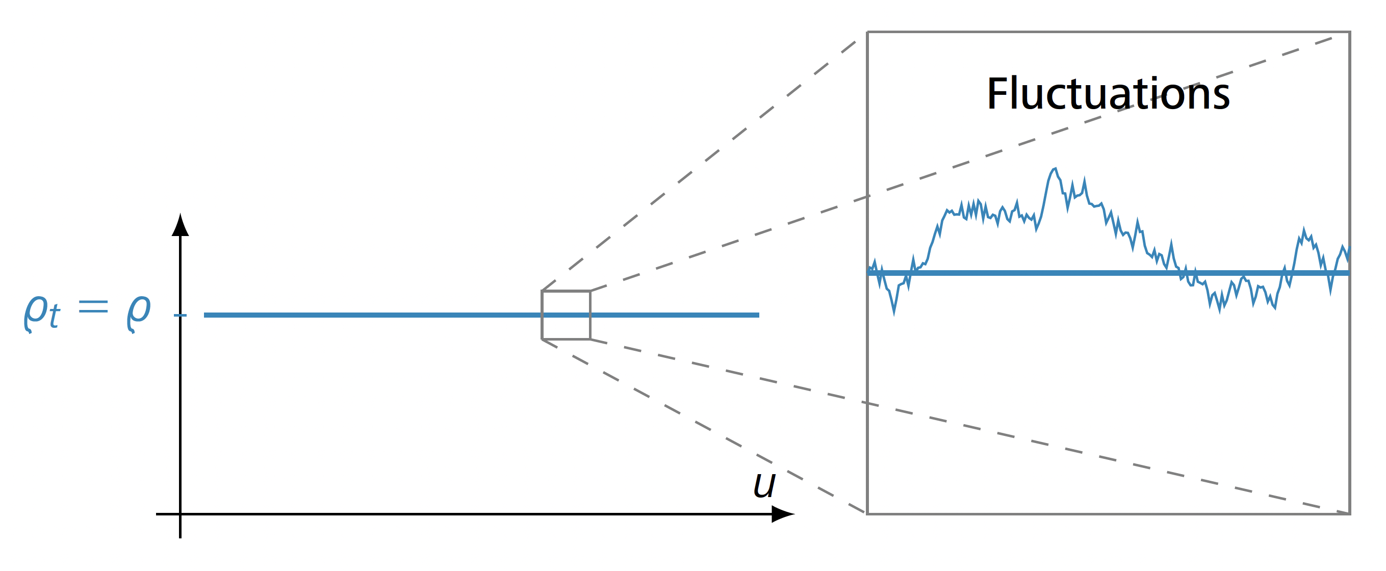
In the last section, we analyzed a Law of Large Numbers for the empirical measure in SIPS with one or more conservation laws. The limit considered in the hydrodynamic limit is deterministic, and we know what is the typical profile that we should observe at any time . The question that we can address now is related to the corresponding Central Limit Theorem, i.e., providing a description of the fluctuations around the hydrodynamic limit. Typically, the study of non-equilibrium fluctuations is very intricate since it requires deep knowledge about the correlations of variables, and this can be quite challenging for the majority of the dynamics. What one is searching for, in the equilibrium scenario in e.g., exclusion processes, is the fluctuations around the constant hydrodynamical profile; see Figure 6.
We start by describing what can happen for systems with a single conservation law and then address the case of more conservation laws.
3.1 Fluctuations for systems with a single conservation law: The exclusion process
As above, first we focus on a system with a single conservation law, the exclusion process, and from now on, we assume that it starts from the stationary state, the Bernoulli product measure of parameter given in (2). We define the empirical field associated to the density, which is the linear functional defined on functions (belonging to a suitable space) as
This expression is obtained by first integrating the test function with respect to the empirical measure in (2), then removing the mean with respect to (2), and finally dividing the result by . The question that arises now is to understand the limit in distribution, as , of , denoted by . For the exclusion processes introduced above, one can get several different limits.
A. For the SSEP and in the diffusive scaling , the Ornstein–Uhlenbeck (OU) process is given by
B. For the WASEP with a weak asymmetry, i.e., and in the diffusive scaling , one gets the same as (9), while for , one gets the Kardar–Parisi–Zhang (KPZ) equation (introduced in [44 M. Kardar, G. Parisi and Y.-C. Zhang, Dynamic scaling of growing interfaces. Phys. Rev. Lett. 56, 889–892 (1986) ]) or its companion, the stochastic Burgers (SB) equation, respectively, for the height field or for the density field ,
Here stands for the standard space-time white noise.
The height field can be defined analogously to the density field, but the relevant quantity for this field is the net flux of particles through the bond ; the definition of the field is as in (8), but with and its average replaced by and the corresponding average.
The results described above were obtained and analyzed in [18 I. Corwin, The Kardar–Parisi–Zhang equation and universality class. Random Matrices Theory Appl. 1, Article ID 1130001 (2012) , 31 P. Gonçalves and M. Jara, Crossover to the KPZ equation. Ann. Henri Poincaré 13, 813–826 (2012) , 32 P. Gonçalves and M. Jara, Nonlinear fluctuations of weakly asymmetric interacting particle systems. Arch. Ration. Mech. Anal. 212, 597–644 (2014) , 33 P. Gonçalves and M. Jara, The Einstein relation for the KPZ equation. J. Stat. Phys. 158, 1262–1270 (2015) , 36 P. Gonçalves, M. Jara and S. Sethuraman, A stochastic Burgers equation from a class of microscopic interactions. Ann. Probab. 43, 286–338 (2015) , 37 P. Gonçalves, M. Jara and M. Simon, Second order Boltzmann–Gibbs principle for polynomial functions and applications. J. Stat. Phys. 166, 90–113 (2017) , 40 M. Gubinelli and M. Jara, Regularization by noise and stochastic Burgers equations. Stoch. Partial Differ. Equ. Anal. Comput. 1, 325–350 (2013) , 41 M. Gubinelli and N. Perkowski, Energy solutions of KPZ are unique. J. Amer. Math. Soc. 31, 427–471 (2018) ] and were extended to many other stationary models in stationarity; recently, some of them have been extended to the non-equilibrium scenario; see [55 K. Yang, Stochastic Burgers equation via energy solutions from non-stationary particle systems, preprint, arXiv:1810.02836 (2018) ].
C. For the ASEP, i.e., and in the hyperbolic scaling ,
Note that if, in this expression, we take , we get a trivial evolution for the density field. The same is true if instead we redefine the field in a frame with the velocity . Therefore, to get a non-trivial behavior, we have to speed up the time, and for the choice , the limit field is given in terms of the so-called KPZ fixed point, which was constructed in [48 K. Matetski, J. Quastel and D. Remenik, The KPZ fixed point. Acta Math. 227, 115–203 (2021) ]. In [30 P. Gonçalves, Central limit theorem for a tagged particle in asymmetric simple exclusion. Stochastic Process. Appl. 118, 474–502 (2008) ], it was proved that, up to the time scale , there is no evolution of the density field, and its law coincides with the law of the initial field . Nevertheless, beyond that time scale, the limit is not yet known, but it should be given in terms of the KPZ fixed point. The results of [30 P. Gonçalves, Central limit theorem for a tagged particle in asymmetric simple exclusion. Stochastic Process. Appl. 118, 474–502 (2008) ] applied to WASEP show that, below the line , there is no time evolution, but in fact, the trivial evolution should go up to the line ; see the gray region on Figure 7.
For a transition probability allowing long jumps, the limit behavior can be Gaussian, or given in terms of a fractional OU (when the symmetry dominates) or of the fractional SB equation (when symmetry and asymmetry have exactly the same strength); see [34 P. Gonçalves and M. Jara, Stochastic Burgers equation from long range exclusion interactions. Stochastic Process. Appl. 127, 4029–4052 (2017) , 35 P. Gonçalves and M. Jara, Density fluctuations for exclusion processes with long jumps. Probab. Theory Related Fields 170, 311–362 (2018) ].
In the case of exclusion processes given by a general transition probability, we have already seen possible laws, given as solutions to stochastic PDEs (SPDEs) governing the fluctuations of the unique conserved quantity, the number of particles. The way to connect one solution to the other could be either by changing the nature of the tail of the transition probability or the symmetry/asymmetry dominance phase of the transition probability. The nature of the SPDE is very much related to the underlying SIPS, but the same equation can be obtained from a variety of different particle models, and in that sense, it is universal.
3.2 Fluctuations for multi-component systems
We observe that the results described in the last subsection are for systems with (only) one conservation law, and for these, there is no ambiguity concerning the choice of the fields that one should look at – the only choice is the field associated to the conserved quantity. When systems have more than one conserved quantity, and their evolution is coupled, as is the case for the ABC model or the interface models that we described above, we have to be careful when we define those fields. Moreover, a special feature of multi-component models is that different time scales coexist, which never occurs for systems with only one conserved quantity.
In [52 H. Spohn, Nonlinear fluctuating hydrodynamics for anharmonic chains. J. Stat. Phys. 154, 1191–1227 (2014) ], with a focus on anharmonic chains of oscillators, the nonlinear fluctuating hydrodynamics theory (NLFH) for the equilibrium time-correlations of the conserved quantities of that model was developed and analytical predictions were done based on a mode-coupling approximation. Roughly speaking, Spohn’s approach starts at the macroscopic level, i.e., one assumes that a hyperbolic system of conservation laws governs the macroscopic evolution of the empirical conserved quantities. Then a diffusion term and a dissipation term are added to the system of coupled PDEs and one linearizes the system at second order with respect to the equilibrium averages of the conserved quantities. A fundamental role is played by the normal modes, i.e., the eigenvectors of the linearized equation. These modes evolve with different velocities and in different time scales. They might be described by different forms of superdiffusion or standard diffusion processes, and this description depends on the values of certain coupling constants. From this approach, many other universality classes arise, besides the Gaussian or the KPZ, already seen in systems with only one conservation law. Despite all the complications that one might face when dealing with multi-component systems, there is a choice of the potential for the interface models described above, for which all the diagram for the fluctuations of its conserved quantities has been obtained. Now we quickly describe it.
The harmonic potential
Consider the generator given in (7), but with the quadratic potential , the harmonic potential. The invariant measures are explicitly given by
where and . In this case, the system conserves two quantities, the energy and the volume ; note that the average with respect to of and is equal to and , respectively. According to NLFH, the quantities that one should analyze are now
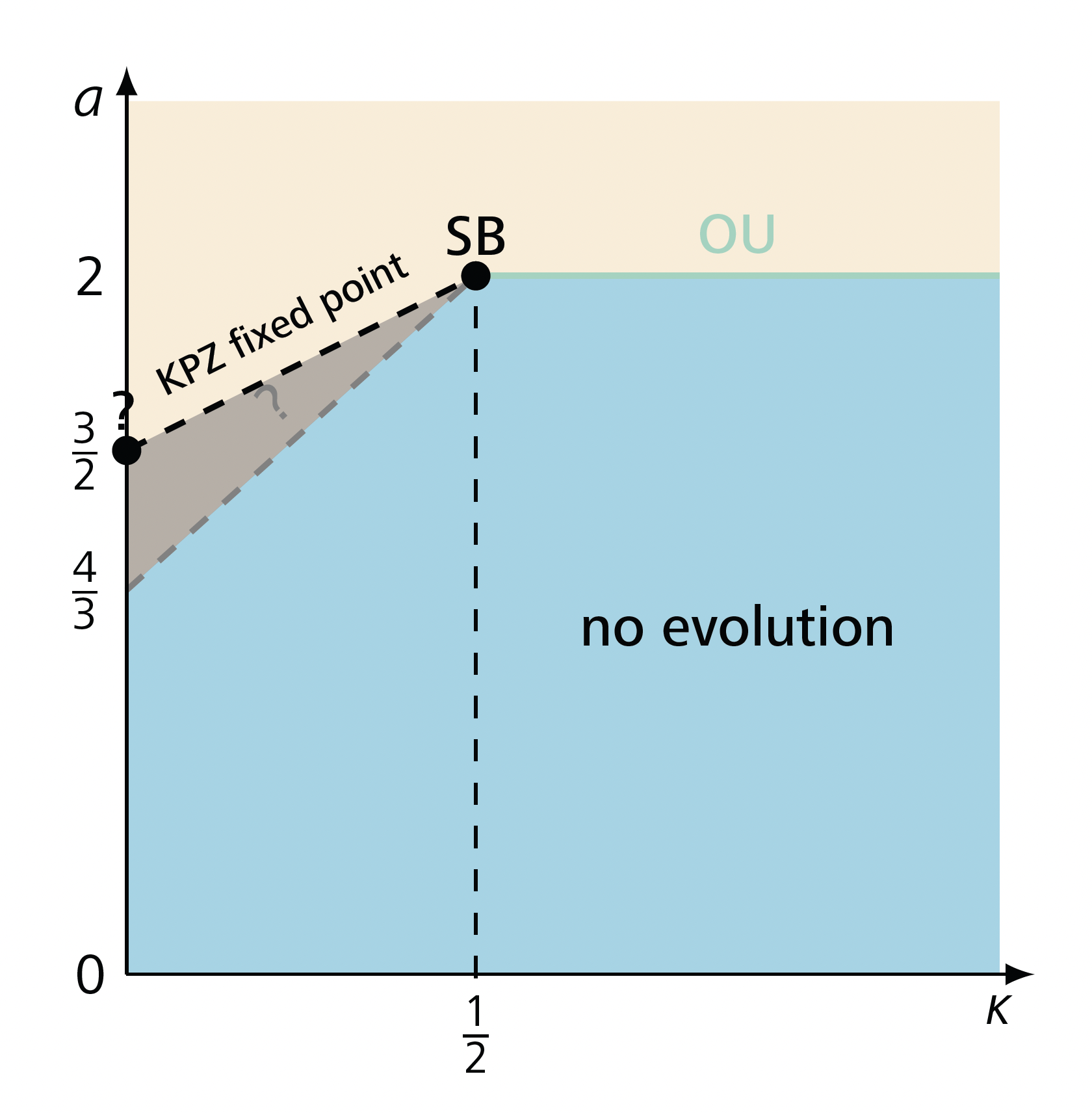
For a random variable , we let denote the centered random variable. Note that, for , we simply get and as the volume and energy, respectively. The corresponding fields should be taken on a frame with velocity and . According to NLFH, in the strong asymmetric regime (), should behave diffusively and should behave as a Lévy process with exponent . For the volume, i.e., the quantity , when we take the fluctuation field with velocity equal to , we get a process that is linearly transported in time (see the light-blue line in Figure 8), while if we take it with the velocity , we get an OU process without drift (see the magenta line).

For with velocity , i.e., the energy (recall that ), we have the results summarized in Figure 9.
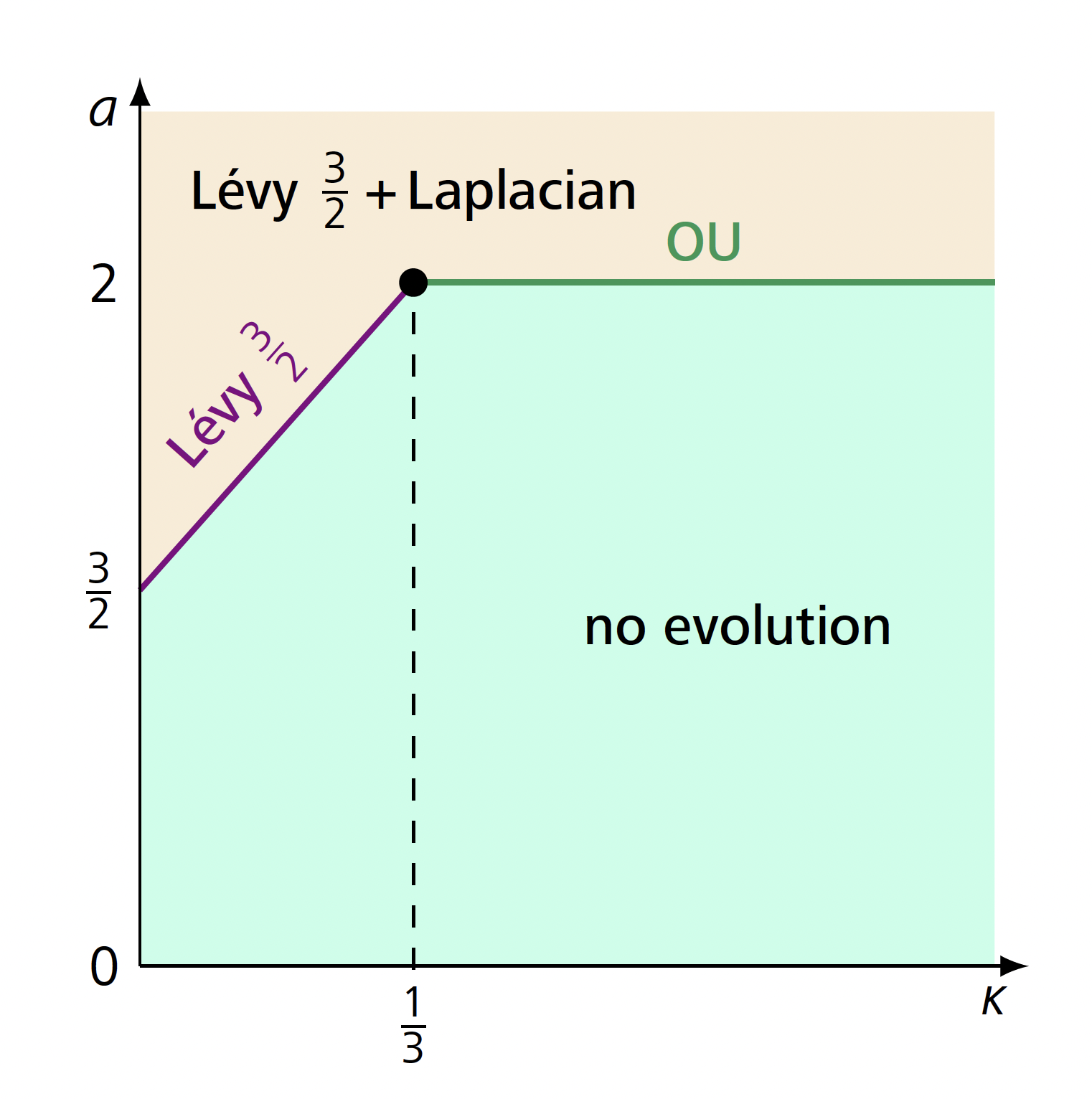
In Figure 8, the light-blue line corresponds to , while the purple line in Figure 9, where we see the Lévy process with exponent , corresponds to . Note that this diagram is complete, but the method that was employed to derive these results relies heavily on the specific form of the dynamics.
There is still much work to do in this direction, and we believe that one should analyze the action of the generator on other relevant quantities and keep track of those that give a non-trivial contribution to the limit. There are several equations that one can obtain from this procedure by using many different microscopic forms of dynamics, and for this reason, they are said to be universal. Understanding how to connect universality classes is a major problem in the field of SIPS. There is much to do regarding this problem, and hopefully, in the next years, large steps will be made in this direction.
4 Final comments
Some of the problems described above were among the goals of the research project titled HyLEF, Hydrodynamic Limits and Equilibrium Fluctuations: universality from stochastic systems, one of the projects funded by the European Research Council (ERC) in the 2016 edition of the ERC Starting Grants. This is the first and so far the only ERC grant awarded in Portugal in the field of mathematics, and it is headed by the author of this article, Patrícia Gonçalves, now a full professor at the mathematics department of Instituto Superior Técnico (IST) of the University of Lisbon. It is a grant of nearly 1.2 million euros for 5 years (extended to 7 years due to the pandemic period) which started on the 1st of December, 2016.
The budget allowed creating a team composed of 4 post-doctoral researchers (2 years each), 2 Ph.D. students (4 years each), and 2 master students (1 year each). This was the first team in Portugal working in the field of SIPS. The budget also allowed organizing conferences and inviting external collaborators to work with the team at IST in Portugal.
I would like to thank the ERC and all the members of the Panel PE1 (Mathematics) who, by selecting my project for funding, have all contributed to a big change in my life and the lives of all the people involved in this project. If HyLEF was not funded by the ERC, the creation of this team under national funds would have been completely impossible.
The group of collaborators of this project includes several researchers, some of them working at the host institution and others working abroad, mainly at IMPA and at the Universities of Arizona, Juelich, Lyon, Nice, among others. Below is a photomontage of some of these members, to whom I am truly grateful for making the last years at IST extremely exciting, not only research-wise, but also personally. I will certainly remember them for a long time.

References
- R. Ahmed, C. Bernardin, P. Gonçalves and M. Simon, A microscopic derivation of coupled SPDE’s with a KPZ flavor. Ann. Inst. Henri Poincaré Probab. Stat. 58, 890–915 (2022)
- C. Bahadoran, Hydrodynamics and hydrostatics for a class of asymmetric particle systems with open boundaries. Comm. Math. Phys. 310, 1–24 (2012)
- R. Baldasso, O. Menezes, A. Neumann and R. R. Souza, Exclusion process with slow boundary. J. Stat. Phys. 167, 1112–1142 (2017)
- C. Bernardin, P. Cardoso, P. Gonçalves and S. Scotta, Hydrodynamic limit for a boundary driven super-diffusive symmetric exclusion, preprint, arXiv:2007.01621 (2021)
- C. Bernardin and P. Gonçalves, Anomalous fluctuations for a perturbed Hamiltonian system with exponential interactions. Comm. Math. Phys. 325, 291–332 (2014)
- C. Bernardin, P. Gonçalves and M. Jara, 3/4-fractional superdiffusion in a system of harmonic oscillators perturbed by a conservative noise. Arch. Ration. Mech. Anal. 220, 505–542 (2016)
- C. Bernardin, P. Gonçalves and M. Jara, Weakly harmonic oscillators perturbed by a conservative noise. Ann. Appl. Probab. 28, 1315–1355 (2018)
- C. Bernardin, P. Gonçalves, M. Jara and M. Simon, Nonlinear perturbation of a noisy Hamiltonian lattice field model: Universality persistence. Comm. Math. Phys. 361, 605–659 (2018)
- C. Bernardin, P. Gonçalves and B. Jiménez-Oviedo, Slow to fast infinitely extended reservoirs for the symmetric exclusion process with long jumps. Markov Process. Related Fields 25, 217–274 (2019)
- C. Bernardin, P. Gonçalves and B. Jiménez-Oviedo, A microscopic model for a one parameter class of fractional Laplacians with Dirichlet boundary conditions. Arch. Ration. Mech. Anal. 239, 1–48 (2021)
- C. Bernardin and G. Stoltz, Anomalous diffusion for a class of systems with two conserved quantities. Nonlinearity 25, 1099–1133 (2012)
- L. Bertini, N. Cancrini and G. Posta, On the dynamical behavior of the ABC model. J. Stat. Phys. 144, 1284–1307 (2011)
- L. Bonorino, R. de Paula, P. Gonçalves and A. Neumann, Hydrodynamics of porous medium model with slow reservoirs. J. Stat. Phys. 179, 748–788 (2020)
- P. Capitão and P. Gonçalves, Hydrodynamics of weakly asymmetric exclusion with slow boundary. In From particle systems to partial differential equations, Springer Proc. Math. Stat. 352, Springer, Cham, 123–148 (2021)
- P. Cardoso, R. De Paula and P. Gonçalves, A microscopic model for the fractional porous medium equation; to appear in Nonlinearity
- P. Cardoso, P. Gonçalves and B. Jiménez-Oviedo, Hydrodynamic behavior of long-range symmetric exclusion with a slow barrier: Diffusive regime; to appear in Ann. Inst. Henri Poincaré Probab. Stat.
- P. Cardoso, P. Gonçalves and B. Jiménez-Oviedo, Hydrodynamic behavior of long-range symmetric exclusion with a slow barrier: Superdiffusive regime; accepted for publication in Ann. Sc. Norm. Super. Pisa Cl. Sci. (5)
- I. Corwin, The Kardar–Parisi–Zhang equation and universality class. Random Matrices Theory Appl. 1, Article ID 1130001 (2012)
- A. De Masi, E. Presutti and E. Scacciatelli, The weakly asymmetric simple exclusion process. Ann. Inst. H. Poincaré Probab. Statist. 25, 1–38 (1989)
- A. De Masi, E. Presutti, D. Tsagkarogiannis and M. E. Vares, Current reservoirs in the simple exclusion process. J. Stat. Phys. 144, 1151–1170 (2011)
- R. De Paula, P. Gonçalves and A. Neumann, Energy estimates and convergence of weak solutions of the porous medium equation. Nonlinearity 34, 7872–7915 (2021)
- C. Erignoux, P. Gonçalves and G. Nahum, Hydrodynamics for SSEP with non-reversible slow boundary dynamics: Part I, the critical regime and beyond. J. Stat. Phys. 181, 1433–1469 (2020)
- C. Erignoux, P. Gonçalves and G. Nahum, Hydrodynamics for SSEP with non-reversible slow boundary dynamics: Part II, below the critical regime. ALEA Lat. Am. J. Probab. Math. Stat. 17, 791–823 (2020)
- M. R. Evans, Y. Kafri, H. M. Koduvely and D. Mukamel, Phase separation in one-dimensional driven diffusive systems. Phys. Rev. Lett. 80, 425–429 (1998)
- M. R. Evans, Y. Kafri, H. M. Koduvely and D. Mukamel, Phase separation and coarsening in one-dimensional driven diffusive systems: Local dynamics leading to long-range Hamiltonians. Phys. Rev. E (3) 58, 2764–2778 (1998)
- C. Franceschini, P. Gonçalves and B. Salvador, Hydrodynamical behavior for the generalized symmetric exclusion with open boundary; to appear in Math. Phys. Anal. Geom.
- T. Franco, P. Gonçalves and A. Neumann, Hydrodynamical behavior of symmetric exclusion with slow bonds. Ann. Inst. Henri Poincaré Probab. Stat. 49, 402–427 (2013)
- T. Franco, P. Gonçalves and A. Neumann, Phase transition of a heat equation with Robin’s boundary conditions and exclusion process. Trans. Amer. Math. Soc. 367, 6131–6158 (2015)
- T. Franco, P. Gonçalves and G. M. Schütz, Scaling limits for the exclusion process with a slow site. Stochastic Process. Appl. 126, 800–831 (2016)
- P. Gonçalves, Central limit theorem for a tagged particle in asymmetric simple exclusion. Stochastic Process. Appl. 118, 474–502 (2008)
- P. Gonçalves and M. Jara, Crossover to the KPZ equation. Ann. Henri Poincaré 13, 813–826 (2012)
- P. Gonçalves and M. Jara, Nonlinear fluctuations of weakly asymmetric interacting particle systems. Arch. Ration. Mech. Anal. 212, 597–644 (2014)
- P. Gonçalves and M. Jara, The Einstein relation for the KPZ equation. J. Stat. Phys. 158, 1262–1270 (2015)
- P. Gonçalves and M. Jara, Stochastic Burgers equation from long range exclusion interactions. Stochastic Process. Appl. 127, 4029–4052 (2017)
- P. Gonçalves and M. Jara, Density fluctuations for exclusion processes with long jumps. Probab. Theory Related Fields 170, 311–362 (2018)
- P. Gonçalves, M. Jara and S. Sethuraman, A stochastic Burgers equation from a class of microscopic interactions. Ann. Probab. 43, 286–338 (2015)
- P. Gonçalves, M. Jara and M. Simon, Second order Boltzmann–Gibbs principle for polynomial functions and applications. J. Stat. Phys. 166, 90–113 (2017)
- P. Gonçalves, C. Landim and C. Toninelli, Hydrodynamic limit for a particle system with degenerate rates. Ann. Inst. Henri Poincaré Probab. Stat. 45, 887–909 (2009)
- P. Gonçalves, R. Misturini and A. Occelli, Hydrodynamics for the ABC model with slow/fast boundary; to appear in Stochastic Process. Appl.
- M. Gubinelli and M. Jara, Regularization by noise and stochastic Burgers equations. Stoch. Partial Differ. Equ. Anal. Comput. 1, 325–350 (2013)
- M. Gubinelli and N. Perkowski, Energy solutions of KPZ are unique. J. Amer. Math. Soc. 31, 427–471 (2018)
- M. Jara, Hydrodynamic limit of particle systems with long jumps, preprint, arXiv:0805.1326 (2008)
- L. Jensen and H.-T. Yau, Hydrodynamical scaling limits of simple exclusion models. In Probability theory and applications (Princeton, NJ, 1996), IAS/Park City Math. Ser. 6, Amer. Math. Soc., Providence, 167–225 (1999)
- M. Kardar, G. Parisi and Y.-C. Zhang, Dynamic scaling of growing interfaces. Phys. Rev. Lett. 56, 889–892 (1986)
- C. Kipnis and C. Landim, Scaling limits of interacting particle systems. Grundlehren Math. Wiss. 320, Springer, Berlin (1999)
- T. M. Liggett, Interacting particle systems. Grundlehren Math. Wiss. 276, Springer, New York (1985)
- C. MacDonald, J. Gibbs and A. Pipkin, Kinetics of biopolymerization on nucleic acid templates. Biopolymer 6, 1–25 (1968)
- K. Matetski, J. Quastel and D. Remenik, The KPZ fixed point. Acta Math. 227, 115–203 (2021)
- S. Sethuraman and D. Shahar, Hydrodynamic limits for long-range asymmetric interacting particle systems. Electron. J. Probab. 23, Paper No. 130 (2018)
- F. Spitzer, Interaction of Markov processes. Advances in Math. 5, 246–290 (1970) (1970)
- H. Spohn, Large scale dynamics of interacting particles. Texts and Monographs in Physics, Springer, Berlin (1991).
- H. Spohn, Nonlinear fluctuating hydrodynamics for anharmonic chains. J. Stat. Phys. 154, 1191–1227 (2014)
- H. Spohn and G. Stoltz, Nonlinear fluctuating hydrodynamics in one dimension: The case of two conserved fields. J. Stat. Phys. 160, 861–884 (2015)
- L. Xu, Hydrodynamics for one-dimensional ASEP in contact with a class of reservoirs. J. Stat. Phys. 189, Paper No. 1 (2022)
- K. Yang, Stochastic Burgers equation via energy solutions from non-stationary particle systems, preprint, arXiv:1810.02836 (2018)
Cite this article
Patrícia Gonçalves, Hydrodynamic limits: The emergence of fractional boundary conditions. Eur. Math. Soc. Mag. 127 (2023), pp. 5–14
DOI 10.4171/MAG/123