
1 Introduction
On 18 October 2013, I was sitting on my living room sofa scrolling through the news, when one article caught my attention. The headline read something along the lines of “Sleep cleans the brain of toxins”, and described a recent original research study from the lab of neuroscientist Prof. Maiken Nedergaard [39 L. Xie, H. Kang, Q. Xu, M. J. Chen, Y. Liao, M. Thiyagarajan, J. O’Donnell, D. J. Christensen, C. Nicholson, J. J. Iliff et al., Sleep drives metabolite clearance from the adult brain. Science 342, 373–377 (2013) ]. In a series of experiments, Nedergaard and her team had injected a fluorescent dye (a so-called tracer or contrast agent) into the fluids surrounding the brain of mice, and observed that the tracer moved into (and out of) the brain many times faster in sleeping mice than in awake mice. Their findings revealed a fundamental interplay between sleep and brain clearance, but also highlighted how far from complete our understanding of the brain’s waterscape (Definition 1) is.
Definition 1. The brain’s waterscape is the circulation, flow and exchange of tissue fluid and associated solute transport through and around the brain.
Our brains are composed of very soft tissue consisting of neurons, glial cells, and interstitial space filled with interstitial fluid (ISF), penetrated by blood vessels, and surrounded by a bath of cerebrospinal fluid (CSF). Its well-being crucially relies on the transport of solutes: the influx of oxygen and nutrients, and clearance of metabolic waste. Due to the barrier layers between blood, tissue and CSF in the brain, the fluid exchange between these spaces is limited and regulated. Tracer experiments act as a proxy for quantifying this fluid flow and exchange, in lack of more direct medical techniques for measuring water movement in-vivo (Figure 1)1All clinical data presented and visualized here courtesy of P. K. Eide and G. Ringstad, Oslo University Hospital – Rikshospitalet.. In the nearly ten years since 2013, the brain’s waterscape has been attracting substantial and increasing interest from the neurocommunity; more about that to follow.
A year before the striking sleep study [39 L. Xie, H. Kang, Q. Xu, M. J. Chen, Y. Liao, M. Thiyagarajan, J. O’Donnell, D. J. Christensen, C. Nicholson, J. J. Iliff et al., Sleep drives metabolite clearance from the adult brain. Science 342, 373–377 (2013) ], Nedergaard had launched a new theory for describing the brain’s waterscape: the glymphatic system [22 J. J. Iliff, M. Wang, Y. Liao, B. A. Plogg, W. Peng et al., A paravascular pathway facilitates CSF flow through the brain parenchyma and the clearance of interstitial solutes, including amyloid β. Sci. Transl. Med. 4, DOI 10.1126/scitranslmed.3003748 (2012) ]. In the original glymphatic concept, CSF enters the brain via perivascular spaces surrounding brain arteries, mixes with ISF and flows in bulk and convectively through the tissue, and ISF is cleared from the brain along perivascular spaces surrounding brain veins. With my background in analysis of numerical methods for partial differential equations describing biological tissue, I was immediately intrigued by this setting. I also quickly realized that this was an underdeveloped area for applied mathematics, and that even fundamental concepts for multiscale modelling of the brain’s waterscape were missing. Fortunately, the European Research Council Mathematics Panel agreed, and funded my project proposal in the summer of 2016.
In the next few years, we very much realized that the brain’s waterscape was even less understood and more discussed that what I had originally thought, and that its mechanisms were surrounded by controversy. It seemed as though almost every piece of the glymphatic theory was disputed with different groups arguing about, e.g., the role of diffusion versus convection, the existence of any convective flow and, if existent, its directionality, the importance vs. nonimportance of aquaporin channels and glial cells, the pathways for clearance, the anatomy of the compartments involved, etc. The list could go on and on. For us, this made the need for mathematical and computational foundations even more obvious to, e.g., quantify observations, bridge between species, and test, reject or support hypotheses.
2 Quantifying brain solute transport
Transport of solutes is often described via the usual convection-diffusion-reaction equation: in a domain () and over a time interval , find the concentration such that
where the subscript denotes the time derivative, and are the divergence and gradient respectively, is the diffusion tensor, is a convective velocity field and is a kinetic reaction rate. In addition, may be prescribed on the boundary for a.e. , and initially for . Numerical approximations of (1) are readily computed using finite difference and finite element methods, via, e.g., the FEniCS software [2 M. Alnæs, J. Blechta, J. Hake, A. Johansson, B. Kehlet, A. Logg, C. Richardson, J. Ring, M. E. Rognes and G. N. Wells, The FEniCS project version 1.5. Archive of Numerical Software 3, 9–23 (2015) ].

2.1 Modelling the glymphatic theory via stochastic fields
Now, in our first step towards modelling human brain solute transport [7 M. Croci, V. Vinje and M. E. Rognes, Uncertainty quantification of parenchymal tracer distribution using random diffusion and convective velocity fields. Fluids Barriers CNS 16, 1–21 (2019) ], we took a just-published clinical study as a starting point [32 G. Ringstad, S. A. S. Vatnehol and P. K. Eide, Glymphatic MRI in idiopathic normal pressure hydrocephalus. Brain 140, 2691–2705 (2017) ]. Ringstad, Vatnehol and Eide [32 G. Ringstad, S. A. S. Vatnehol and P. K. Eide, Glymphatic MRI in idiopathic normal pressure hydrocephalus. Brain 140, 2691–2705 (2017) ] had injected a contrast agent into the fluid-filled spaces surrounding the spine, and then imaged its whereabouts within the brain 1–48 hours later (Figure 1). They concluded that it seems unlikely that diffusion alone explains the brain-wide distribution. We asked: “is it?” and were curious as to whether mathematical modelling could support, quantify and/or add to this statement.
Stochastic diffusion
First, in order to quantify the unlikeliness of diffusion as a sole mechanism, a key question was how to capture the uncertainty associated with the brain’s diffusivity as a random field. Importantly, we aimed to ensure that diffusivity samples were positive, with a literature-based expected value , and appropriate variability. To this end, we represented as a continuous random field
where for each fixed , is a gamma-distributed random variable with a prescribed shape () and scaling (). To also enforce continuity and to effectively sample the diffusion field, we drew samples of by first sampling a Matérn field (with a given smoothness and correlation length), and then mapping it onto a gamma random field via a copula (see, e.g., [7 M. Croci, V. Vinje and M. E. Rognes, Uncertainty quantification of parenchymal tracer distribution using random diffusion and convective velocity fields. Fluids Barriers CNS 16, 1–21 (2019) ] and references therein for further details). Next, we pieced together inputs from several sources: a human brain finite element mesh with nearly two million vertices and ten million cells, and a upwards-travelling contrast agent distribution on the mesh boundary based on an eye-norm estimation of the published data [32 G. Ringstad, S. A. S. Vatnehol and P. K. Eide, Glymphatic MRI in idiopathic normal pressure hydrocephalus. Brain 140, 2691–2705 (2017) ].
In short, we found that the uncertainty in the diffusion field magnitude had a substantial impact on the amount of contrast agent both in the grey and white matter. While the clinically observed distribution of contrast in the grey matter was well within the expected variability of diffusion, its distribution into the white matter was not. We could thus support the claim that diffusion was likely not sufficient as a sole mechanism, but at the same time highlight that diffusion was likely nearly sufficient. Further, we demonstrated that local variations (i.e., heterogeneity) in the diffusion field had little impact on expected values, and thus that contrast agent distribution in larger brain regions could be well approximated by average diffusion coefficients.
Stochastic convection
We next asked how we could represent the convective velocity described by the glymphatic theory in a stochastic setting at the brain scale? Well,
varies more after a distance proportional to the mean distance between arterioles and venules ( mm);
the vasculature is random and independent of space in the sense that the presence of paraarterial or paravenous spaces are equally likely at any point in space (hence the expected value of each is zero);
is continuous and ; and
older experimental studies indicate an expected velocity magnitude µm/s with some variability.
In turn, we defined the stochastic glymphatic circulation velocity field as the curl of three standard independent identically distributed Matérn fields with correlation length and scaled to align with the expected value and variability. Then, again using Monte Carlo simulations, we computed samples via (4), but now with non-zero s.
Surprisingly (or perhaps not), we found that the expected tracer distribution with or without the glymphatic velocity were nearly identical and with little variability. Thus, on average, small fluctuations in the CSF/ISF velocity did not increase (or decrease) the influx or clearance of contrast agent in the brain on a larger scale. Indeed, further model variations, such as including a directional flow at the macroscale and allowing for local fluid influx and/or efflux, were required for the convective terms to effectively contribute to the solute transport [7 M. Croci, V. Vinje and M. E. Rognes, Uncertainty quantification of parenchymal tracer distribution using random diffusion and convective velocity fields. Fluids Barriers CNS 16, 1–21 (2019) ].
Remark 2. Despite its limitations, this uncertainty quantification study felt like a true breakthrough: we had taken advantage of an original mathematical approach and produced new physiologically relevant insights. Importantly, it was the first study by my team that had been accepted and published in Fluids and Barriers of the Central Nervous System, a domain-specific journal read by everyone and anyone interested in brain mechanics, including neurosurgeons and neuroradiologists, neuroscientists, biophysicists, bioengineers (and mathematicians).
Remark 3. Another, more mathematical, question is how to sample Matérn field efficiently, especially in the context of more advanced Monte Carlo methods over non-trivial geometries. As such, this physiological problem setting also guided us to develop new sampling and Monte Carlo algorithms [8 M. Croci, V. Vinje and M. E. Rognes, Fast uncertainty quantification of tracer distribution in the brain interstitial fluid with multilevel and quasi Monte Carlo. Int. J. Numer. Methods Biomed. Eng. 37, Paper No. e3412 (2021) ].
2.2 Identifying convective flow: An inverse problem
With these insights, we understood more about the roles and properties of diffusion and convection via CSF/ISF flow within the brain. We also understood that in order to get much further, we needed a closer collaboration with the clinicians and better access to the raw data. Luckily, Prof. P.-K. Eide and Dr. G. Ringstad at Oslo University Hospital were very willing to share their data and expertise with us and very enthusiastic about exploring how computational modelling could contribute to quantify and interpret their clinical findings.
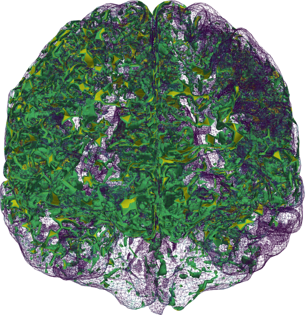
We then found ourselves in the unprecedented position of having multi-modal magnetic resonance (MR) data, including T1- and T2-weighted structural images, T1-maps, diffusion tensor images and contrast MR images, available for several individual in different cohorts. MR data are characteristically at high spatial resolution, but only available at a sparse set of discrete time points, e.g., hours after contrast injection. These images combined allowed us to segment and construct subject-specific finite element meshes, interpolate subject-specific diffusion tensor fields (Figure 2 (a)), and map MR contrast signal intensities onto finite element concentration fields for each subject and each time point (Figure 1).
Remark 4. In fact, to handle this data set, we developed and published an open-source pipeline going from magnetic resonance brain images to finite element simulations, accompanied by an open-access introductory booklet [25 K.-A. Mardal, M. E. Rognes, T. B. Thompson and L. M. Valnes, Mathematical modeling of the human brain: From MRI to finite element simulation. Springer (2022) ].
An optical flow problem?
Now, given this data set, could we identify and quantify the convective flow of ISF/CSF within the brain? Or the task in more mathematical terms: given non-negative scalar fields , identify a transport field that maps onto in a (to be defined) suitable sense.
This is a classical problem setting, known in computer vision as the optical flow problem [21 B. K. Horn and B. G. Schunck, Determining optical flow. Artif. Intell. 17, 185–203 (1981) ]. The idea is that given at for , find an optimal that minimizes an objective functional ,
In the original optical flow setting, it is assumed that maps to by convective transport alone – corresponding to
and the initial and final conditions , . The choice of regularization term (and also for that matter) gives variations of the method; one option is to minimize the kinetic energy:
This formulation yields the -Monge–Kantorovich mass transfer problem, analysed across three centuries (see [3 J.-D. Benamou and Y. Brenier, A computational fluid mechanics solution to the Monge–Kantorovich mass transfer problem. Numer. Math. 84, 375–393 (2000) ] and references therein), and used by Tannenbaum, Ratner et al. [30 V. Ratner, L. Zhu, I. Kolesov, M. Nedergaard, H. Benveniste and A. Tannenbaum, Optimal-mass-transfer-based estimation of glymphatic transport in living brain. In Medical Imaging 2015: Image Processing, SPIE (2015) ] early on to study mouse brain transport via in-vivo imaging.
However, when we applied this method to our human image data set, we quickly faced several challenges. First, by considering transport by convection alone (3), we ignore the substantial contribution from diffusion. Second, we found the method sensitive to the choice of the regularization parameter . And third, locally, for which (2) is not obviously well posed. We therefore needed to develop a more physiologically accurate and more numerically robust approach.
Bilinear flow control
Still targeting the task of “given at , identify a convective flow field defined over the time interval ”, we instead considered the bilinear optimal control problem of finding minimizers
subject to , and such that (1) holds (with ) over . We let , though that choice can easily be reevaluated. Note that we deliberately allow for non-divergence-free velocity fields in light of our previous results (Section 2.1) indicating that local fluid influx and efflux may be key for effective convective transport. This problem setting is very similar to that studied in terms of well-posedness and existence by Glowinski et al. [20 R. Glowinski, Y. Song, X. Yuan and H. Yue, Bilinear optimal control of an advection-reaction-diffusion system. SIAM Rev. 64, 392–421 (2022) ] modulo choice of regularization and incompressibility (divergence-free) constraint (or lack thereof).
There are two main approaches to solving the constrained minimization problem (4): either (i) introducing a Lagrange multiplier for the PDE-constraint and solving the resulting nonlinear Euler–Lagrange problems directly (the all-at-once approach), or (ii) iteratively solving the optimization problem by solving the PDE-constraint (1) with as initial condition for a series of by means, e.g., a quasi-Newton method (the reduced approach). After numerical experiments and comparisons, we found that the latter approach (using an L-BFGS algorithm) was more robust for our uses in the sense that this method successfully converged for most patients and time intervals between brain scans and yielded consistent results for different mesh resolutions and values of the regularization parameters.
Remark 5. Our previous work on automated solution of high-dimensional inverse problems and accompanying software dolfin-adjoint [18 P. E. Farrell, D. A. Ham, S. W. Funke and M. E. Rognes, Automated derivation of the adjoint of high-level transient finite element programs. SIAM J. Sci. Comput. 35, C369–C393 (2013) , 2 M. Alnæs, J. Blechta, J. Hake, A. Johansson, B. Kehlet, A. Logg, C. Richardson, J. Ring, M. E. Rognes and G. N. Wells, The FEniCS project version 1.5. Archive of Numerical Software 3, 9–23 (2015) ] proved to be very useful here.
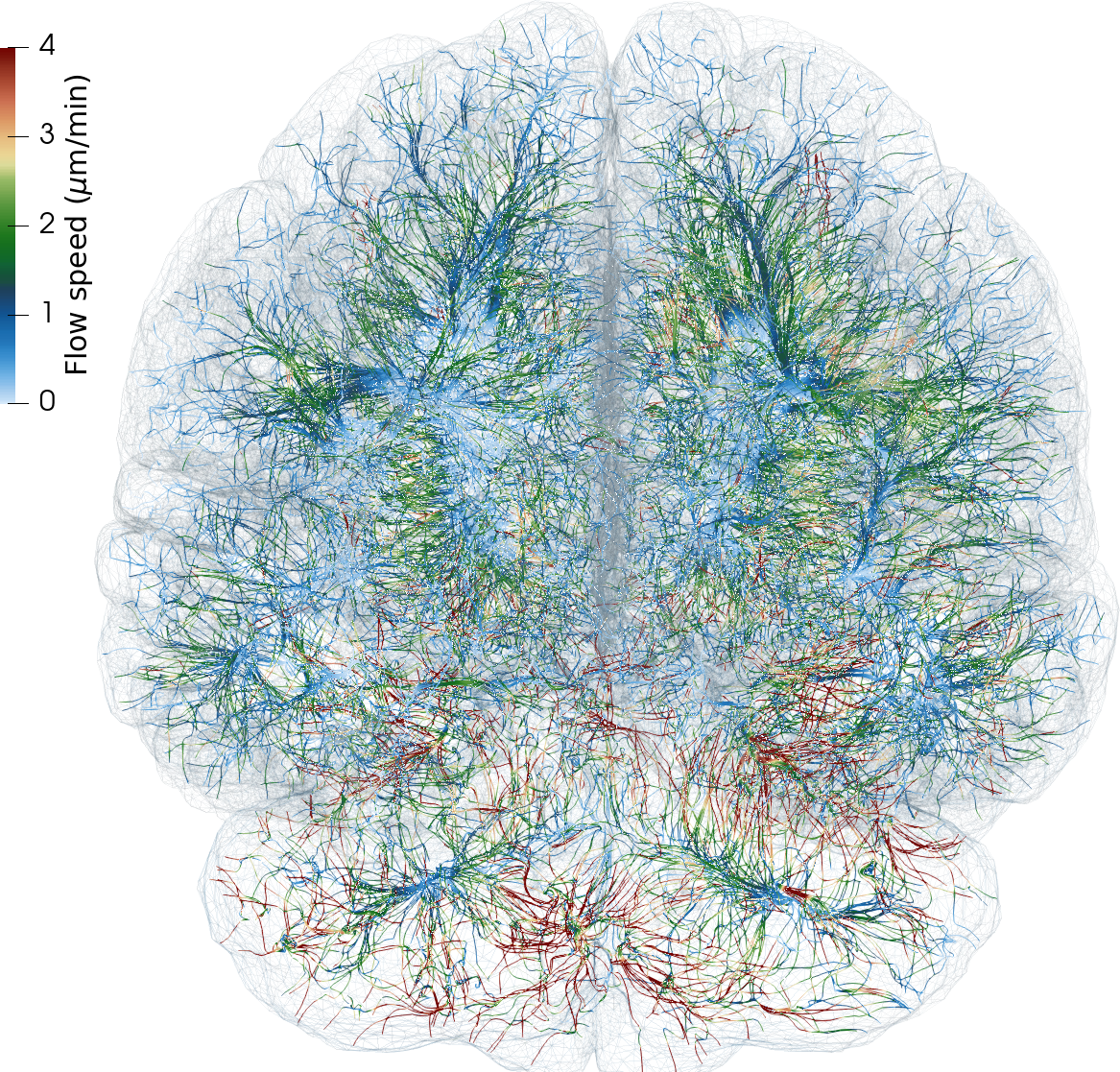
Ultimately, we thus decided to estimate net (time-averaged) velocity fields in the contrast agent influx phase h and clearance phase h for each patient by solving (4) (using subject-specific finite element meshes, diffusion tensors and concentration observations) via a reduced approach using a fixed maximal number of iterations (Figure 2 (b)). Interestingly, for all subjects and time intervals, we identified persistent velocity fields with brain-averaged velocity magnitudes (i.e., flow speeds) of 1–8 µm/min. These flow speeds correspond to bulk flow rates of 0.1–0.8 µL/(g min) – a range which compares fascinatingly well with estimated bulk flow rates of 0.1–0.3 µL/(g min) from early (1970s–80s) tracer experiments in cats [1 N. J. Abbott, Evidence for bulk flow of brain interstitial fluid: Significance for physiology and pathology. Neurochem. Int. 45, 545–552 (2004) ]. Interestingly, we can also estimate the net fluid influx/efflux by computing, e.g., the brain-wide average of , and find that water dominantly flows into the brain (e.g., by filtration from the blood stream) at a rate of 1–4 min.
Open problem 6. Our findings suggest that high-dimensional inverse modelling offers a powerful avenue of investigation for the brain’s waterscape. However, a question that remains is how well-posed the optimization problem is with respect to the uncertainty in the input data and choice of regularization functional. Moreover, clearly there are “terra incognita” (or perhaps rather “mare incognita”) for which there is little information in the medical images, i.e., little or no contrast agent present, and where velocity field estimates intuitively would be associated with substantial uncertainty. Quantifying the uncertainty and information level required for reliable flow estimates in this setting is a open problem.
So, using stochastic and inverse modelling as described, we have quantified the relative contributions of diffusion and convection in brain solute transport, suggesting that these modes coexist and co-contribute. The next question is: given that there is a persistent convective fluid flow within the brain parenchyma, what could be the mechanisms and the brain mechanics allowing for such a flow?
3 The brain as a pulsating poroelastic medium
From the viewpoint of mechanics, the brain is an almost surprisingly soft elastic medium, enclosed and protected by the stiffer meninges and much stiffer skull, and permeated by a number of fluid networks including the blood-filled vasculature (arteries, capillaries and veins), the ISF-filled extracellular space between brain cells, and potential CSF- or ISF-filled perivascular spaces surrounding the vasculature. With every heart beat (the cardiac rhythm) and breath (the respiratory cycle), your brain expands and contracts with displacements of the order of 1 mm and volume changes of the order of 1 cm. The precise interplay and transfer of forces and sources between these compartments, and how these change with age and disorders, still lacks understanding and quantification however.
In pioneering work, Tully and Ventikos [34 B. Tully and Y. Ventikos, Cerebral water transport using multiple-network poroelastic theory: Application to normal pressure hydrocephalus. J. Fluid Mech. 667, 188–215 (2011) ] introduced the multiple-network poroelastic theory (MPET), a theory originating in fractured geological reservoirs, in the context of modelling brain solid and fluid mechanics. Specifically, the quasi-static MPET equations enforce balance of momentum and mass and read as: for a given number of networks , (), and a time interval find the displacement field and the -th network pressure field for such that
Here is the elastic stress-strain relationship and describes the transfer of mass between fluid networks. In the linear and isotropic case,
with Lamé parameters and . Each network is equipped with its Biot–Willis coefficient with , its storage coefficient , and its hydraulic conductivity tensor , while the network interactions are described via the exchange coefficients . We also note that the fluid (Darcy) velocity in network is defined by
For simplicity, consider the basic boundary conditions , on and initial conditions here.
In the case , the MPET equations reduce to Biot’s equations, whose properties have been studied for decades (and still actively are). The general MPET equations however seemed to have received much less attention from the mathematical community.
3.1 MPET as an elliptic-parabolic problem
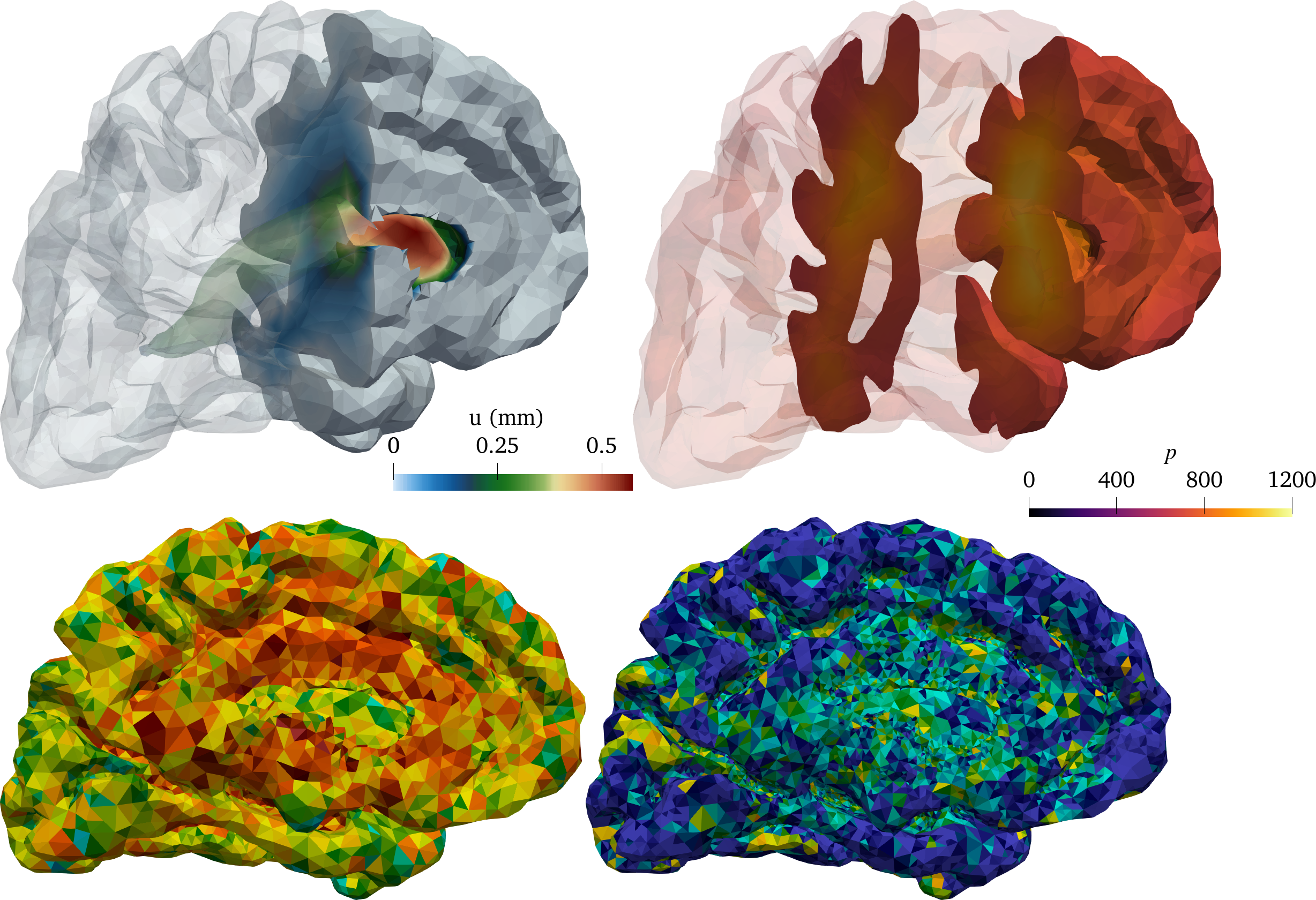
To analyse approximations of the MPET equations (Figure 3), we realized that the framework of coupled elliptic-parabolic problems as introduced by Ern and Meunier [17 A. Ern and S. Meunier, A posteriori error analysis of Euler–Galerkin approximations to coupled elliptic-parabolic problems. M2AN Math. Model. Numer. Anal. 43, 353–375 (2009) ] provided an ideal starting point. Specifically, this framework considers variational problems in space and time of the form “given bilinear forms , , , and and input data and , find and such that, for almost every ,
with the initial condition ”. Crucially, under natural assumptions on the bilinear forms and the underlying (Hilbert) spaces, and subsequently spatial and temporal discretizations, Ern and Meunier [17 A. Ern and S. Meunier, A posteriori error analysis of Euler–Galerkin approximations to coupled elliptic-parabolic problems. M2AN Math. Model. Numer. Anal. 43, 353–375 (2009) ] derived optimal stability estimates, a priori error estimates and a posteriori error estimates for such problems.
Introducing , and denoting and analogously for , the MPET equations (5) take the form of a coupled elliptic-parabolic problem (7) via the identifications
Clearly, and as defined are Hilbert spaces, dense in and , respectively, is symmetric, continuous and coercive if , ), is continuous for and is symmetric, continuous and coercive for . By assuming that the exchange coefficients are positive, symmetric , and bounded, and that the conductivities are bounded (including from below: ), shuffling terms and the Poincaré inequality gives that is symmetric, coercive and continuous, then stability and uniqueness follows for (weak) solutions of the MPET equations (5) [17 A. Ern and S. Meunier, A posteriori error analysis of Euler–Galerkin approximations to coupled elliptic-parabolic problems. M2AN Math. Model. Numer. Anal. 43, 353–375 (2009) ].
Introducing a conforming finite element discretization of and relative to a mesh with mesh size and a first-order implicit time discretization with time steps to define discrete approximations and , a priori and a posteriori error estimates (Figure 3) also follow.
For solutions and approximations of the MPET equations, and for each time step , ,
where are a posteriori computable quantities involving appropriately weighted cell and facet residual contributions, and are determined by the approximation of the initial data and source terms, respectively.
3.2 The incompressible MPET equations
As the human brain is composed of 80 % water, it is widely considered (nearly) incompressible ( in (5)). It therefore seems highly relevant to ask if the variational formulation (7) with forms given by (8) and the estimates of Theorem 7 are robust with respect to ? The answer is no: the continuity of the linear elasticity form (and thus the error estimates) degenerate as . Indeed, it is illuminating to take a look at the structure of the MPET equations in this scenario. Set to reveal the extreme cases. As , , the MPET equations decouple into a coupled Darcy flow system for and an elliptic equation for ,
We can thus expect finite element discretization of the MPET equations in the incompressible limit to be wrought with analogous challenges as for the linear elasticity equations.
How should we remedy this situation? An appealing solution, first introduced in the context of Biot’s equations, is to introduce the total pressure as a new variable, . Then the action of the MPET operator transforms into
This formulation is indeed robust in the incompressible limit with energy estimates uniform in and (subsequently a priori error estimates for stable discretizations):
Given sufficiently regular , and initial conditions , solutions , to system (5) satisfy an energy estimate of the form
with inequality constant independent of the parameter .
Preconditioning by congruence
When next turning to the efficient solution of the MPET equations via preconditioned iterative methods, an interesting puzzle appeared with a charming solution motif [27 E. Piersanti, J. J. Lee, T. Thompson, K.-A. Mardal and M. E. Rognes, Parameter robust preconditioning by congruence for multiple-network poroelasticity. SIAM J. Sci. Comput. 43, B984–B1007 (2021) , 28 E. Piersanti, M. E. Rognes and K.-A. Mardal, Parameter robust preconditioning for multi-compartmental Darcy equations. In Numerical mathematics and advanced applications—ENUMATH 2019, Lect. Notes Comput. Sci. Eng. 139, Springer, Cham, 703–711 (2021) ]. To illustrate, consider a coupled Darcy flow with exchange system like (9) written as
where and
Block-diagonal preconditioners of this system easily yield condition numbers that grow with the ratio between the exchange and conductance coefficients [28 E. Piersanti, M. E. Rognes and K.-A. Mardal, Parameter robust preconditioning for multi-compartmental Darcy equations. In Numerical mathematics and advanced applications—ENUMATH 2019, Lect. Notes Comput. Sci. Eng. 139, Springer, Cham, 703–711 (2021) ]. But, can the task of constructing block-diagonal preconditioners be simplified by a linear change of variables with a matrix (1em)?
By definition, a matrix is diagonalizable by congruence if and only if there exists a matrix such that is diagonal. Further, two matrices and are simultaneously diagonalizable by congruence if there exists a matrix such that both and are diagonal. Now, if is a real, symmetric and positive definite and is a real symmetric matrix, then and are simultaneously diagonalizable by congruence. In our case, is symmetric and positive definite as long as and is symmetric; therefore, and are simultaneously diagonalizable by congruence.
Next, in general, if has distinct eigenvalues with eigenvectors , then the matrix constructed from these eigenvectors diagonalizes and by congruence. This observation gives a direct construction for in terms of the eigenvectors of . The transformed system is then block-diagonal and easily preconditioned with condition numbers that are uniform for a range of exchange and conductance parameters [28 E. Piersanti, M. E. Rognes and K.-A. Mardal, Parameter robust preconditioning for multi-compartmental Darcy equations. In Numerical mathematics and advanced applications—ENUMATH 2019, Lect. Notes Comput. Sci. Eng. 139, Springer, Cham, 703–711 (2021) ]. Interestingly, the construction extends to the MPET system [27 E. Piersanti, J. J. Lee, T. Thompson, K.-A. Mardal and M. E. Rognes, Parameter robust preconditioning by congruence for multiple-network poroelasticity. SIAM J. Sci. Comput. 43, B984–B1007 (2021) ].

3.3 Brain-CSF interactions
Remark 9. The total pressure formulation of the MPET equations is also advantageous when considering the fluid-structure interaction between the poroelastic brain and the CSF that surrounds it and clinical applications (Figure 4) [6 M. Causemann, V. Vinje and M. E. Rognes, Human intracranial pulsatility during the cardiac cycle: A computational modelling framework. Fluids Barriers CNS 19, 863–874 (2022) ]. The intracranial pressure, a key clinical measure, can be interpreted as the total pressure in the parenchyma and the hydrostatic pressure in the CSF.
Open problem 10. In-vivo imaging options for brain pulsatility (deformations, stresses) are currently limited, but new techniques such as, e.g., magnetic resonance encephalography (MREG) are coming into play. The quantification of MREG images remains somewhat enigmatic however, and we envision that computational fluid-structure poroelastic brain simulations could provide new interpretations.
3.4 Impermeability and minimal Biot–Stokes stability
The permeability of the brain’s extracellular space is estimated to be of the order 10 nm, which is many orders of magnitude lower than, e.g., the permeability of the blood circulation. Thus, another limit of interest for studying brain fluid flow is the impermeable case . This is a particularly interesting case, often attempted addressed by introducing the Darcy velocity (as defined by (6)) as a separate field.
Taking the (time-discrete) Biot equations (i.e., (5) with ) and as an example; these form a generalized saddle-point system that in the limit as reduces to the incompressible Stokes equations in terms of and . On the other hand as noted previously (cf. (9)), in the limit as , the Biot equations decouple into an elliptic equation for and a (mixed) Darcy equation for ( and) . These observations hint at close relations between Stokes, Darcy, Biot and MPET equations, and suggest that, for combinations of finite element spaces , that the pairing is Stokes stable and Darcy stable in the discrete Babuška–Brezzi sense. However, in the limit at , it is highly non-trivial to ensure uniform Darcy stability [24 K.-A. Mardal, M. E. Rognes and T. B. Thompson, Accurate discretization of poroelasticity without Darcy stability: Stokes–Biot stability revisited. BIT 61, 941–976 (2021) ].
Fortunately, we could show that a revised notion, coined minimal Stokes–Biot stability is sufficient.
Definition 11 (Minimal Stokes–Biot stability [24 K.-A. Mardal, M. E. Rognes and T. B. Thompson, Accurate discretization of poroelasticity without Darcy stability: Stokes–Biot stability revisited. BIT 61, 941–976 (2021) ]). A family of discrete spaces with , and is called minimally Stokes–Biot stable if and only if
the bilinear form is continuous and coercive on ;
are Stokes stable in the discrete Babuška–Brezzi sense;
for each .
Minimally stable Stokes–Biot discrete solutions at each time step converge,
for (depending on regularity, order, etc.), where
Now, returning to the physiology at hand, the moderate pressure differences observed clinically and the nearly vanishing permeability of the extracellular space suggest that extracellular fluid flow is negligible. Could there be alternative, more permeable pathways within the brain?
4 Perivascular fluid flow and model reduction
As the brain lacks lymphatic vessels, fluid-filled spaces surrounding blood vessels – the perivascular spaces (PVSs) – are conjectured to act as higher-permeability proxy pathways; “highways” for fluid efflux and metabolic solute clearance [31 M. L. Rennels, T. F. Gregory, O. R. Blaumanis, K. Fujimoto and P. A. Grady, Evidence for a ‘paravascular’ fluid circulation in the mammalian central nervous system, provided by the rapid distribution of tracer protein throughout the brain from the subarachnoid space. Brain Res. 326, 47–63 (1985) , 22 J. J. Iliff, M. Wang, Y. Liao, B. A. Plogg, W. Peng et al., A paravascular pathway facilitates CSF flow through the brain parenchyma and the clearance of interstitial solutes, including amyloid β. Sci. Transl. Med. 4, DOI 10.1126/scitranslmed.3003748 (2012) ]. At this mesoscale ( mm, s), the vasculature and perivasculature form slender dual networks, running along the brain’s surface and diving into the brain. While experimental studies indicate that solutes move rapidly in PVSs, a lingering question is “what are the mechanisms, characteristics and forces underlying PVS fluid flow”?
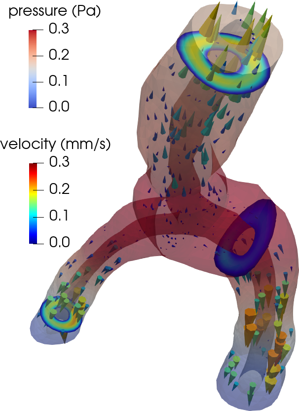
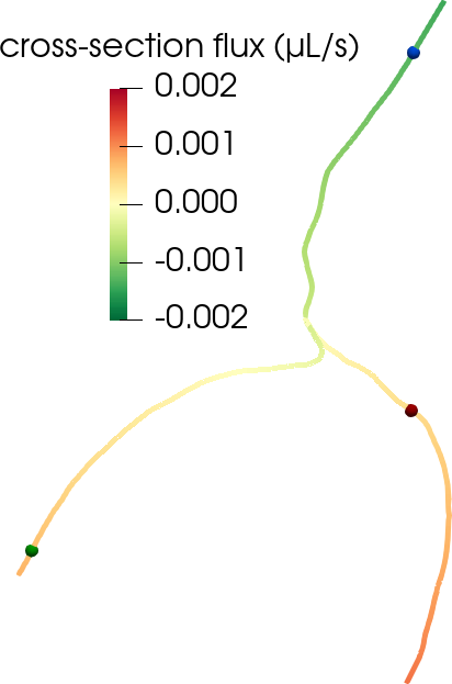
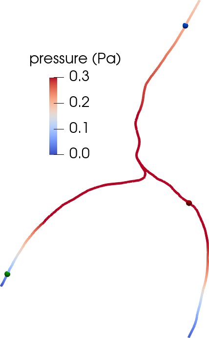
Flow in perivascular spaces appears synchronized with the cardiac cycle. This observation has led to the widespread notion that perivascular flow is driven by arterial wall motion. However, can pulsatile wall motions be a driver for net flow at this scale? To investigate, we created computational models of an annular perivascular segment surrounding an image-based bifurcating blood vessel (Figure 5) and induced laminar (Stokes) flow in the moving PVS by (i) travelling pulse waves on the (inner) blood vessel wall, (ii) pulsatile pressure differences at inlet and outlets, and (iii) static pressure differences. Wall pulsations induce substantial pulsatile flow, but only negligible net flow (due to their long wavelength of 100 mm) [11 C. Daversin-Catty, V. Vinje, K.-A. Mardal and M. E. Rognes, The mechanisms behind perivascular fluid flow. PLOS ONE 15, Paper No. e0244442 (2020) ]. On the other hand, even a small static hydrostatic pressure difference can induce net flow of relevant magnitudes. Such hydrostatic pressure differences could be induced by experimental procedures [37 V. Vinje, A. Eklund, K.-A. Mardal, M. E. Rognes and K.-H. Støverud, Intracranial pressure elevation alters CSF clearance pathways. Fluids Barriers CNS 17, 1–19 (2020) ], but are also of comparable magnitude as transient pressure differences measured in the human brain [38 V. Vinje, G. Ringstad, E. K. Lindstrøm, L. M. Valnes, M. E. Rognes, P. K. Eide and K.-A. Mardal, Respiratory influence on cerebrospinal fluid flow: A computational study based on long-term intracranial pressure measurements. Sci. Rep. 9, 1–13 (2019) ].

Another disputed point is whether there is a net efflux of ISF along perivenous spaces. The original glymphatic theory emphasizes this concept, as injected tracers were observed along arteries, but not around veins at early time points, and along veins at later time points [22 J. J. Iliff, M. Wang, Y. Liao, B. A. Plogg, W. Peng et al., A paravascular pathway facilitates CSF flow through the brain parenchyma and the clearance of interstitial solutes, including amyloid β. Sci. Transl. Med. 4, DOI 10.1126/scitranslmed.3003748 (2012) ]. However, could an alternative explanation for this be connected to the geometry of brain surface arteries and veins? We created pressure-driven Stokes flow models as well as convection-diffusion models of tracer transport from optical coherence tomography images of perivascular spaces surrounding arteries and veins to investigate [36 V. Vinje, E. N. Bakker and M. E. Rognes, Brain solute transport is more rapid in periarterial than perivenous spaces. Sci. Rep. 11, 1–11 (2021) ]. PVS flow speeds were 2–6 times higher in the periarterial geometries than in perivenous geometries (Figure 6). Interestingly, these differences in flow speeds due to geometrical differences (area, shape) lead to delayed tracer transport by about 25–30 min, in agreement with the originally observed delayed tracer distribution surrounding veins.
4.1 Perivascular spaces as topologically 1d-networks
Modelling the interplay between blood vessels and tissue via geometrically reduced models has been an active and important research topic for decades, cf., e.g., [5 L. Cattaneo and P. Zunino, Computational models for fluid exchange between microcirculation and tissue interstitium. Netw. Heterog. Media 9, 135–159 (2014) ] and references therein. In the brain, the characteristic dual networks formed by the cerebral vasculature and perivasculature define a new setting for geometrically reduced fluid flow modelling [9 C. Daversin-Catty, I. G. Gjerde and M. E. Rognes, Geometrically reduced modelling of pulsatile flow in perivascular networks. Front. Phys. (Lausanne), DOI 10.3389/fphy.2022.882260 (2022) ].
Consider a perivascular domain defined as the union of generalized annular cylinder branches . Assume that each such cylinder has a well-defined, oriented, and topologically one-dimensional centreline with coordinate , and let (Figure 5). The set of bifurcation points i.e., the points at which the centrelines of branches meet is denoted . Finally, assume that the boundaries pulsate with a wall speed in the normal direction.
Under a set of assumptions on the moving geometries (axial symmetry, radial boundary movement and fixed centreline) and flow and pressure fields (axial symmetry, constant cross-section pressure, axial velocity profile), we can derive a reduced system of equations for the cross-section flux and average cross-section pressure over time on each centreline with inner and outer radius , (denoting by and by ),
where
In (11), is the density of the fluid and its viscosity, denotes the cross-section area, while is a lumped flow parameter that depends on the domain geometry and the choice of axial velocity profile. We also define the (one-dimensional) normal stress induced by and as
which corresponds to an average of the axial (-)component of the normal stress in each cross-section.
At the bifurcation points , we impose conservation of flux and continuity of normal stress,
where and , represent centrelines of the parent and daughter branches meeting at the bifurcation point , and the respective coordinates of .
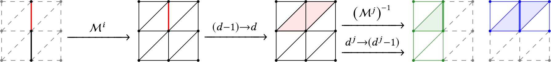
This system is particularly amenable for a variational finite element formulation imposing the flux conservation condition weakly using a Lagrange multiplier. Relative to a finite element mesh of the centreline composed of mesh segments (one for each centreline branch ), we define the
flux space as the space of continuous piecewise quadratics over for each ,
pressure space as the space of continuous piecewise linears on , and
Lagrange multiplier space .
The discrete problem then reads as follows: for each discrete time and time step , find , and solving
for all , , and . Here, is defined by
where , and (and ) is simply the (or 1em) corresponding to the point , and the natural jump is
This formulation provides an inexpensive and reasonably accurate framework for estimating pulsatile perivascular fluid flow in large networks, and thus establishes a mathematical foundation for future computational studies of perivascular flow and transport (Figure 5) [9 C. Daversin-Catty, I. G. Gjerde and M. E. Rognes, Geometrically reduced modelling of pulsatile flow in perivascular networks. Front. Phys. (Lausanne), DOI 10.3389/fphy.2022.882260 (2022) ].
Open problem 13. Originally, I was planning on coupling the vasculature and perivascular spaces with the tissue via topologically one-dimensional dual networks embedded in the three-dimensional volume, see e.g., [5 L. Cattaneo and P. Zunino, Computational models for fluid exchange between microcirculation and tissue interstitium. Netw. Heterog. Media 9, 135–159 (2014) ]. Due to the controversy regarding the existence of flow in brain PVSs and extracellular space, we did not go further with this approach, and as such it remain as (at least) an interesting mathematical problem.
5 Bridging electrochemistry and fluid mechanics
When you are thinking about the brain, the first thing that comes to mind is probably not brain fluid flow. Indeed, neuroscience is possibly foremost occupied with the electrical signalling of the brain. These signals are however generated by electric potential differences, which in turn are induced by ion concentration differences [29 R. Rasmussen, J. O’Donnell, F. Ding and M. Nedergaard, Interstitial ions: A key regulator of state-dependent neural activity? Prog. Neurobiol. 193, DOI 10.1016/j.pneurobio.2020.101802 (2020) ]. On the other hand, differences in ion concentrations also induce water movement by osmosis. Thus, up till now, we have only considered one (mechanical) piece of the puzzle, while ignoring electrical and chemical effects. The challenge is that
the coupling between electrochemical effects, fluid transport and elastic deformation is particularly difficult and is only little understood, specifically in the brain [19 A. Goriely, M. G. Geers, G. A. Holzapfel, J. Jayamohan, A. Jérusalem, S. Sivaloganathan, W. Squier et al., Mechanics of the brain: Perspectives, challenges, and opportunities. Biomech. Model. Mechanobiol. 14, 931–965 (2015) ].
By a pure serendipity, just as we were getting ready to address this challenge, Mori [26 Y. Mori, A multidomain model for ionic electrodiffusion and osmosis with an application to cortical spreading depression. Phys. D 308, 94–108 (2015) ] published an elegant and comprehensive multidomain tissue-level model ionic electrodiffusion and osmotic water flow in biological tissue. In this framework, the tissue domain is composed on coexisting compartments (for instance neuronal, glial, and extracellular spaces) with interacting ionic species (such as sodium Na, potassium K, chloride Cl). The coupled, time-dependent, nonlinear system of PDEs describes the volume fractions , ion concentrations for , electric potentials , mechanical pressures , and fluid velocities for each compartment (see [26 Y. Mori, A multidomain model for ionic electrodiffusion and osmosis with an application to cortical spreading depression. Phys. D 308, 94–108 (2015) , 13 A. J. Ellingsrud, N. Boullé, P. E. Farrell and M. E. Rognes, Accurate numerical simulation of electrodiffusion and water movement in brain tissue. Math. Med. Biol. 38, 516–551 (2021) ]). For instance, in compartments , the movement of each ion concentration is governed by , where is the ion flux density and is the transmembrane water flux between the compartments and . Coupling (chemical) diffusion, drift due to the electric field, as well as fluid flow within each compartment, yields ion fluxes of the form
see the aforementioned references for a complete description.

The combination of diffusion, nonlinear reaction and convection dynamics makes this a highly interesting system to approximate numerically using, e.g., finite element or spectral methods [13 A. J. Ellingsrud, N. Boullé, P. E. Farrell and M. E. Rognes, Accurate numerical simulation of electrodiffusion and water movement in brain tissue. Math. Med. Biol. 38, 516–551 (2021) ]. Moreover, the underlying physiology induces sharp wave fronts that require a very fine spatial and fine temporal resolution for all current methods (Figure 7). As such, the numerical simulation of ionic electrodiffusion and water movement remains a real challenge, and solution approaches that retain accuracy at lower computational expense could enable further uptake in the community.
Remark 14. As the Waterscales project nears its end, it has been rewarding to observe its trajectory from roots in numerical analysis, rapid impact of poroelasticity and fluid dynamics in brain mechanics, and stretching toward impact in neuroscience in the long run. Our most recent work [15 A. J. Ellingsrud, D. B. Dukefoss, R. Enger, G. Halnes, K. Pettersen and M. E. Rognes, Validating a computational framework for ionic electrodiffusion with cortical spreading depression as a case study. eNeuro 9, DOI 10.1523/ENEURO.0408-21.2022 (2022) ] took us back to the project’s origins, by realizing a collaboration with medical experimentalists at the GliaLab at the University of Oslo involved in the development of the original glymphatic theory, while its publication in eNeuro points towards a closer relation with the neuroscience community.
Remark 15. Another question is whether the tissue level is the appropriate scale for modelling the interplay between electrical, chemical and mechanical effects. Indeed, we can envision a paradigm for modelling excitable tissue at the level of cells instead, with explicit representation of cell membranes and spaces. This is however a story for another day [35 A. Tveito, K.-A. Mardal and M. E. Rognes, Modeling excitable tissue: The EMI framework. Simula SpringerBriefs Comput., Rep. Comput. Physiol. 7, Springer, Cham (2021) , 14 A. J. Ellingsrud, C. Daversin-Catty and M. E. Rognes, A cell-based model for ionic electrodiffusion in excitable tissue. In Modeling excitable tissue: The EMI framework, edited by A. Tveito, K.-A. Mardal and M. E. Rognes, Simula SpringerBriefs Comput., Rep. Comput. Physiol. 7, Springer, Cham, 14–27 (2021) ].
6 Computational abstractions and algorithms
Over the last decades, we have witnessed a tremendous increase in the physical, mathematical, numerical and computational complexity of models for physiological processes. To keep up, there has been a corresponding change in how algorithms and software frameworks for the numerical solution of (partial) differential equations are designed. In the context of finite element methods, the FEniCS Project provides a computational platform combining high-level abstractions for the specification of discrete variational formulations with automated code generation of optimized kernels [2 M. Alnæs, J. Blechta, J. Hake, A. Johansson, B. Kehlet, A. Logg, C. Richardson, J. Ring, M. E. Rognes and G. N. Wells, The FEniCS project version 1.5. Archive of Numerical Software 3, 9–23 (2015) , 18 P. E. Farrell, D. A. Ham, S. W. Funke and M. E. Rognes, Automated derivation of the adjoint of high-level transient finite element programs. SIAM J. Sci. Comput. 35, C369–C393 (2013) ]. However, FEniCS support for multidomain, multiscale and/or multiphysics problems has been sorely lacking.
A core Waterscales aim was to remedy this situation by designing numerical algorithms and software abstractions that allow for high-level specification and high-performance forward and reverse solution of models with multiscale features. We addressed this goal by designing and introducing mathematical software concepts together with lower-level algorithms for expressing, representing, and solving systems of PDEs coupled across interfaces or subdomains (Figure 8) [10 C. Daversin-Catty, C. N. Richardson, A. J. Ellingsrud and M. E. Rognes, Abstractions and automated algorithms for mixed domain finite element methods. ACM Trans. Math. Software 47, Article No. 31, DOI 10.1145/3471138 (2021) ]. These tools enable automated assembly and solution of a wide range of mixed finite element variational formulations, such as, e.g., the finite element spaces and formulations involved in the reduced perivascular flow models (11), interactions across the cell membrane in geometrically resolved models of excitable tissue [35 A. Tveito, K.-A. Mardal and M. E. Rognes, Modeling excitable tissue: The EMI framework. Simula SpringerBriefs Comput., Rep. Comput. Physiol. 7, Springer, Cham (2021) , 16 A. J. Ellingsrud, A. Solbrå, G. T. Einevoll, G. Halnes and M. E. Rognes, Finite element simulation of ionic electrodiffusion in cellular geometries. Front. Neuroinf., DOI 10.3389/fninf.2020.00011 (2020) ] or fluid-structure interfaces [6 M. Causemann, V. Vinje and M. E. Rognes, Human intracranial pulsatility during the cardiac cycle: A computational modelling framework. Fluids Barriers CNS 19, 863–874 (2022) ]. All algorithms are publicly and openly available via the FEniCS Project software [2 M. Alnæs, J. Blechta, J. Hake, A. Johansson, B. Kehlet, A. Logg, C. Richardson, J. Ring, M. E. Rognes and G. N. Wells, The FEniCS project version 1.5. Archive of Numerical Software 3, 9–23 (2015) , 10 C. Daversin-Catty, C. N. Richardson, A. J. Ellingsrud and M. E. Rognes, Abstractions and automated algorithms for mixed domain finite element methods. ACM Trans. Math. Software 47, Article No. 31, DOI 10.1145/3471138 (2021) ].
Open problem 16. High-level computational specification and automated solution of, e.g., coupled -dimensional problems (), such as to represent interactions between the (peri)vasculature and CSF or tissue, comes with an additional set of challenges including, e.g., non-conforming averaging and extension operators and computational geometry classification problems, and remains an open problem.
7 Brain clearance and neurodegeneration
All-in-all, why are we really so interested in solute transport in the human brain? Well, there are two intertwined clinical reasons – either to transport treatment drugs into the brain, or to understand how metabolic waste clears from the brain – in order to better comprehend and hopefully treat neurodegenerative diseases such as, e.g., Alzheimer’s disease.
With new and quantitative physiological insights at hand, we could now mathematically describe the role of dynamical clearance in the propagation of toxic proteins across the brain. Representing the brain’s connectome (i.e., fiber bundle pathways) by a graph , we study the distribution of the protein concentrations and regional clearance values (), evolving via the graph Laplacian that describes anisotropic diffusion and nonlinear reactions as
with initial conditions on ; here are kinetic parameters, and and critical and minimal clearance values, respectively [4 G. S. Brennan, T. B. Thompson, H. Oliveri, M. E. Rognes and A. Goriely, The role of clearance in neurodegenerative disease. bioRxiv, DOI 10.1101/2022.03.31.486533 (2022) ].
The local () dynamical system (12) admits a class of “healthy” fixed points for any , stable for , and also unconditionally stable, “unhealthy” fixed points . The full system describes intriguing pathways of toxic protein propagation and clearance decay (Figure 9) in which the dynamic clearance waterscapes alter disease progression [4 G. S. Brennan, T. B. Thompson, H. Oliveri, M. E. Rognes and A. Goriely, The role of clearance in neurodegenerative disease. bioRxiv, DOI 10.1101/2022.03.31.486533 (2022) ].
8 Concluding remarks and outlook
In my original project proposal, I wrote that Waterscales would be bridging the fluid mechanics across scales and electrophysiology of the brain – with ample opportunities for further mathematical, numerical and more applied study. Indeed, the brain’s waterscape has proven to be a rich field for applied and computational mathematics, which we have only begun to explore. We have many more questions, both in terms of mathematics and physiology, now than when we started. An important interdisciplinary lesson has been that medicine is not mathematics: uncertainties prevail and a single published experiment or clinical study is not “proof” nor settles a case once and for all. However, we have successfully created new mathematical models, new numerical methods, new computational technology and new physiological insights, and importantly, a vibrant research environment targeting ground-breaking research in computational brain electromechanics ready for new challenges.
- 1
All clinical data presented and visualized here courtesy of P. K. Eide and G. Ringstad, Oslo University Hospital – Rikshospitalet.
References
- N. J. Abbott, Evidence for bulk flow of brain interstitial fluid: Significance for physiology and pathology. Neurochem. Int. 45, 545–552 (2004)
- M. Alnæs, J. Blechta, J. Hake, A. Johansson, B. Kehlet, A. Logg, C. Richardson, J. Ring, M. E. Rognes and G. N. Wells, The FEniCS project version 1.5. Archive of Numerical Software 3, 9–23 (2015)
- J.-D. Benamou and Y. Brenier, A computational fluid mechanics solution to the Monge–Kantorovich mass transfer problem. Numer. Math. 84, 375–393 (2000)
- G. S. Brennan, T. B. Thompson, H. Oliveri, M. E. Rognes and A. Goriely, The role of clearance in neurodegenerative disease. bioRxiv, DOI 10.1101/2022.03.31.486533 (2022)
- L. Cattaneo and P. Zunino, Computational models for fluid exchange between microcirculation and tissue interstitium. Netw. Heterog. Media 9, 135–159 (2014)
- M. Causemann, V. Vinje and M. E. Rognes, Human intracranial pulsatility during the cardiac cycle: A computational modelling framework. Fluids Barriers CNS 19, 863–874 (2022)
- M. Croci, V. Vinje and M. E. Rognes, Uncertainty quantification of parenchymal tracer distribution using random diffusion and convective velocity fields. Fluids Barriers CNS 16, 1–21 (2019)
- M. Croci, V. Vinje and M. E. Rognes, Fast uncertainty quantification of tracer distribution in the brain interstitial fluid with multilevel and quasi Monte Carlo. Int. J. Numer. Methods Biomed. Eng. 37, Paper No. e3412 (2021)
- C. Daversin-Catty, I. G. Gjerde and M. E. Rognes, Geometrically reduced modelling of pulsatile flow in perivascular networks. Front. Phys. (Lausanne), DOI 10.3389/fphy.2022.882260 (2022)
- C. Daversin-Catty, C. N. Richardson, A. J. Ellingsrud and M. E. Rognes, Abstractions and automated algorithms for mixed domain finite element methods. ACM Trans. Math. Software 47, Article No. 31, DOI 10.1145/3471138 (2021)
- C. Daversin-Catty, V. Vinje, K.-A. Mardal and M. E. Rognes, The mechanisms behind perivascular fluid flow. PLOS ONE 15, Paper No. e0244442 (2020)
- E. Eliseussen, M. E. Rognes and T. B. Thompson, A-posteriori error estimation and adaptivity for multiple-network poroelasticity, preprint, arXiv:2111.13456 (2021)
- A. J. Ellingsrud, N. Boullé, P. E. Farrell and M. E. Rognes, Accurate numerical simulation of electrodiffusion and water movement in brain tissue. Math. Med. Biol. 38, 516–551 (2021)
- A. J. Ellingsrud, C. Daversin-Catty and M. E. Rognes, A cell-based model for ionic electrodiffusion in excitable tissue. In Modeling excitable tissue: The EMI framework, edited by A. Tveito, K.-A. Mardal and M. E. Rognes, Simula SpringerBriefs Comput., Rep. Comput. Physiol. 7, Springer, Cham, 14–27 (2021)
- A. J. Ellingsrud, D. B. Dukefoss, R. Enger, G. Halnes, K. Pettersen and M. E. Rognes, Validating a computational framework for ionic electrodiffusion with cortical spreading depression as a case study. eNeuro 9, DOI 10.1523/ENEURO.0408-21.2022 (2022)
- A. J. Ellingsrud, A. Solbrå, G. T. Einevoll, G. Halnes and M. E. Rognes, Finite element simulation of ionic electrodiffusion in cellular geometries. Front. Neuroinf., DOI 10.3389/fninf.2020.00011 (2020)
- A. Ern and S. Meunier, A posteriori error analysis of Euler–Galerkin approximations to coupled elliptic-parabolic problems. M2AN Math. Model. Numer. Anal. 43, 353–375 (2009)
- P. E. Farrell, D. A. Ham, S. W. Funke and M. E. Rognes, Automated derivation of the adjoint of high-level transient finite element programs. SIAM J. Sci. Comput. 35, C369–C393 (2013)
- A. Goriely, M. G. Geers, G. A. Holzapfel, J. Jayamohan, A. Jérusalem, S. Sivaloganathan, W. Squier et al., Mechanics of the brain: Perspectives, challenges, and opportunities. Biomech. Model. Mechanobiol. 14, 931–965 (2015)
- R. Glowinski, Y. Song, X. Yuan and H. Yue, Bilinear optimal control of an advection-reaction-diffusion system. SIAM Rev. 64, 392–421 (2022)
- B. K. Horn and B. G. Schunck, Determining optical flow. Artif. Intell. 17, 185–203 (1981)
- J. J. Iliff, M. Wang, Y. Liao, B. A. Plogg, W. Peng et al., A paravascular pathway facilitates CSF flow through the brain parenchyma and the clearance of interstitial solutes, including amyloid β. Sci. Transl. Med. 4, DOI 10.1126/scitranslmed.3003748 (2012)
- J. J. Lee, E. Piersanti, K.-A. Mardal and M. E. Rognes, A mixed finite element method for nearly incompressible multiple-network poroelasticity. SIAM J. Sci. Comput. 41, A722–A747 (2019)
- K.-A. Mardal, M. E. Rognes and T. B. Thompson, Accurate discretization of poroelasticity without Darcy stability: Stokes–Biot stability revisited. BIT 61, 941–976 (2021)
- K.-A. Mardal, M. E. Rognes, T. B. Thompson and L. M. Valnes, Mathematical modeling of the human brain: From MRI to finite element simulation. Springer (2022)
- Y. Mori, A multidomain model for ionic electrodiffusion and osmosis with an application to cortical spreading depression. Phys. D 308, 94–108 (2015)
- E. Piersanti, J. J. Lee, T. Thompson, K.-A. Mardal and M. E. Rognes, Parameter robust preconditioning by congruence for multiple-network poroelasticity. SIAM J. Sci. Comput. 43, B984–B1007 (2021)
- E. Piersanti, M. E. Rognes and K.-A. Mardal, Parameter robust preconditioning for multi-compartmental Darcy equations. In Numerical mathematics and advanced applications—ENUMATH 2019, Lect. Notes Comput. Sci. Eng. 139, Springer, Cham, 703–711 (2021)
- R. Rasmussen, J. O’Donnell, F. Ding and M. Nedergaard, Interstitial ions: A key regulator of state-dependent neural activity? Prog. Neurobiol. 193, DOI 10.1016/j.pneurobio.2020.101802 (2020)
- V. Ratner, L. Zhu, I. Kolesov, M. Nedergaard, H. Benveniste and A. Tannenbaum, Optimal-mass-transfer-based estimation of glymphatic transport in living brain. In Medical Imaging 2015: Image Processing, SPIE (2015)
- M. L. Rennels, T. F. Gregory, O. R. Blaumanis, K. Fujimoto and P. A. Grady, Evidence for a ‘paravascular’ fluid circulation in the mammalian central nervous system, provided by the rapid distribution of tracer protein throughout the brain from the subarachnoid space. Brain Res. 326, 47–63 (1985)
- G. Ringstad, S. A. S. Vatnehol and P. K. Eide, Glymphatic MRI in idiopathic normal pressure hydrocephalus. Brain 140, 2691–2705 (2017)
- M. E. Rognes, T. B. Thompson and E. Eliseussen, A-posteriori error estimation and adaptivity for multiple-network poroelasticity (unpublished)
- B. Tully and Y. Ventikos, Cerebral water transport using multiple-network poroelastic theory: Application to normal pressure hydrocephalus. J. Fluid Mech. 667, 188–215 (2011)
- A. Tveito, K.-A. Mardal and M. E. Rognes, Modeling excitable tissue: The EMI framework. Simula SpringerBriefs Comput., Rep. Comput. Physiol. 7, Springer, Cham (2021)
- V. Vinje, E. N. Bakker and M. E. Rognes, Brain solute transport is more rapid in periarterial than perivenous spaces. Sci. Rep. 11, 1–11 (2021)
- V. Vinje, A. Eklund, K.-A. Mardal, M. E. Rognes and K.-H. Støverud, Intracranial pressure elevation alters CSF clearance pathways. Fluids Barriers CNS 17, 1–19 (2020)
- V. Vinje, G. Ringstad, E. K. Lindstrøm, L. M. Valnes, M. E. Rognes, P. K. Eide and K.-A. Mardal, Respiratory influence on cerebrospinal fluid flow: A computational study based on long-term intracranial pressure measurements. Sci. Rep. 9, 1–13 (2019)
- L. Xie, H. Kang, Q. Xu, M. J. Chen, Y. Liao, M. Thiyagarajan, J. O’Donnell, D. J. Christensen, C. Nicholson, J. J. Iliff et al., Sleep drives metabolite clearance from the adult brain. Science 342, 373–377 (2013)
- B. Zapf, V. Vinje, G. Ringstad, P. K. Eide, M. E. Rognes and K.-A. Mardal, High-dimensional inverse modelling of transport in the human brain, personal communication (2022)
Cite this article
Marie E. Rognes, Waterscales: Mathematical and computational foundations for modelling cerebral fluid flow. Eur. Math. Soc. Mag. 126 (2022), pp. 13–26
DOI 10.4171/MAG/115