
The present column is devoted to Differential Equations.
I Six new problems – solutions solicited
Solutions will appear in a subsequent issue.
260
Let be a -differentiable and convex function with .
Prove that, for every , the following inequality holds:
Determine all functions for which we have equality.
Dorin Andrica (“Babeş-Bolyai” University, Cluj-Napoca, Romania) and Mihai Piticari (“Dragoş Vodă” National College, Câmpulung Moldovenesc, Romania)
261
Let be the unknown function of the following fractional-order derivative Cauchy problem:
Find the solution of this problem by solving an equivalent first-order ordinary Cauchy problem, with a solution independent on the kernel of the fractional operator.
Carlo Cattani (Engineering School, DEIM, University “La Tuscia”, Viterbo, Italy)
262
Let be the unknown function of the following Bernoulli fractional-order Cauchy problem:
where is a continuous function in the interval .
Find the solution of this problem by solving an equivalent first-order ordinary Cauchy problem, with a solution independent on the kernel of the fractional operator. Carlo Cattani (Engineering School, DEIM, University “La Tuscia”, Viterbo, Italy)
263
Let be a real-valued -function defined on , strictly increasing, such that for all and . Consider the boundary value problem
Prove that the solution has exactly one zero in , i.e., there exists a unique point such that , and give a positive lower bound for . Luz Roncal (BCAM – Basque Center for Applied Mathematics, Bilbao, Spain, Ikerbasque Basque Foundation for Science, Bilbao, Spain and Universidad del País Vasco/Euskal Herriko Unibertsitatea, Bilbao, Spain)
264
We propose an interesting stochastic-source scattering problem in acoustics. The stochastic nature for such problems forces us to deal with stochastic partial differential equations (SPDEs), rather than the partial differential equations (PDEs) which hold for the corresponding deterministic counterparts. In particular, we provide the appropriate variational formulation for the stochastic-source Helmholtz equation.
We consider the following boundary value problem (BVP) for the Helmholtz equation with a stochastic source:
where is a generalized stochastic source and
are stochastic Hermite polynomials with , being a probability space. The Hermite polynomials are denoted by , whereas the tensor product is denoted by . We also define the Hermite functions as follows:
and we set , where is related to the following tensor products:
with and . In addition, we employ the countable index , and there only finitely many .
For the stochastic problem (1), we use the expansions
to get a hierarchy of deterministic BVPs
Assume that solves problem (2). Then prove that, for every , the solution satisfies
George Kanakoudis, Konstantinos G. Lallas and Vassilios Sevroglou (Department of Statistics and Insurance Science, University of Piraeus, Piraeus 18534, Greece)
265
For a Newtonian incompressible fluid, the Navier–Stokes momentum equation, in vector form, reads [3 M. A. Xenos, An Euler–Lagrange approach for studying blood flow in an aneurysmal geometry. Proc. A. 473, 20160774 (2017) ]
Here, is the fluid density, is the velocity vector field, is the pressure, is the viscosity, and is an external force field.
(i) Assuming that both the pressure drop and the external field are negligible, it is easy to show that equation (3) reduces to
and finally to equation (4), where is the so-called kinematic viscosity [4 M. A. Xenos and A. C. Felias, Nonlinear dynamics of the KdV-B equation and its biomedical applications. In Nonlinear Analysis, Differential Equations, and Applications, Springer Optim. Appl. 173, Springer, Cham, 765–793 (2021) ].
(ii) Regarding the one-dimensional viscous Burgers equation
prove that an analytical solution can be obtained by means of the Tanh Method [1 W. Malfliet and W. Hereman, The tanh method. I. Exact solutions of nonlinear evolution and wave equations. Phys. Scripta 54, 563–568 (1996) , 2 A.-M. Wazwaz, The tanh method for traveling wave solutions of nonlinear equations. Appl. Math. Comput. 154, 713–723 (2004) , 4 M. A. Xenos and A. C. Felias, Nonlinear dynamics of the KdV-B equation and its biomedical applications. In Nonlinear Analysis, Differential Equations, and Applications, Springer Optim. Appl. 173, Springer, Cham, 765–793 (2021) ] as
M. A. Xenos and A. C. Felias (Department of Mathematics, University of Ioannina, Greece)
II Open problems
(A) Uniqueness of positive steady states for KPP equations in general domains
by Henri Berestycki (Centre d’analyse et de mathématique sociales, EHESS-CNRS, Paris, France; Institute for Advanced Study, Hong Kong University of Science and Technology)
Reaction-diffusion equations
These arise ubiquitously in the modelling of population dynamics, and more generally in biology and ecology. Remarkably, various fields converge on these equations. In addition to modelling in the life sciences and, of course, nonlinear partial differential equations, they arise in probability theory (via branching particle systems) and statistical physics. These equations have witnessed remarkable progress in recent years. Yet, many basic problems remain open. The object of this note is to present a couple of such questions that are simple to formulate.
Reaction-diffusion equations of homogeneous type read in general as in . The nonlinear term is called the reaction term and the Laplacian operator is associated with diffusion. This equation is termed homogeneous because it does not involve explicitly the location (or time ) and also because it is set in all of space. The Fisher–KPP case (or strong KPP case) refers to the class of nonlinear terms of class that satisfy
The archetypal example is . These reactions terms were introduced and first studied by Fisher [13 R. A. Fisher, The wave of advance of advantageous genes. Ann. Eugen. 7, 355–369 (1937) ] and Kolmogorov, Petrovsky and Piskunov (KPP) [14 A. N. Kolmogorov, I. G. Petrovsky and N. S. Piskunov, Étude de l’équation de la diffusion avec croissance de la quantité de matière et son application à un problème biologique. Bull. Univ. Moskow, Ser. Internat., Sec. A 1, 1–25 (1937) ]. I will discuss some questions related to the uniqueness of bounded positive stationary solutions, that is, bounded positive solutions of the semilinear elliptic equation with boundary conditions.
Heterogeneous equations
In recent years, many works have addressed heterogeneous versions of the equations introduced above. These arise in various guises. First, the reaction term is allowed to vary in space and time: . Likewise, in various models, one wishes to consider more general second-order elliptic operators than the Laplacian:
My works with Hamel and Rossi [10 H. Berestycki, F. Hamel and L. Rossi, Liouville-type results for semilinear elliptic equations in unbounded domains. Ann. Mat. Pura Appl. (4) 186, 469–507 (2007) ] and Hamel and Nadin [8 H. Berestycki, F. Hamel and G. Nadin, Asymptotic spreading in heterogeneous diffusive excitable media. J. Funct. Anal. 255, 2146–2189 (2008) ] are devoted precisely to this type of question. The interested reader will find in or infer from these papers open problems analogous to several that I describe here.
Another natural heterogeneity arises from the geometry of the domain of propagation when it is not the whole space. Given an open subset subject to Dirichlet boundary conditions, we are led to study the problem
Indeed, in many cases of interest, for all , and then one can show that any non-negative bounded solution (besides 0) satisfies .
Existence
To discuss the existence of a positive solution of (6), we use the generalized principal Dirichlet eigenvalue in the domain , defined as
This definition coincides in the present case with the notion of generalized principal eigenvalue introduced in [11 H. Berestycki, L. Nirenberg and S. R. S. Varadhan, The principal eigenvalue and maximum principle for second-order elliptic operators in general domains. Comm. Pure Appl. Math. 47, 47–92 (1994) ] and applied to unbounded domains in [12 H. Berestycki and L. Rossi, Generalizations and properties of the principal eigenvalue of elliptic operators in unbounded domains. Comm. Pure Appl. Math. 68, 1014–1065 (2015) ]. We can then state the existence result in a more general framework of weak KPP class:
Existence in (6) is conditioned by this eigenvalue.
Let satisfy the weak KPP condition (7). Then (6) admits a positive bounded solution if Conversely, if , (6) has no positive bounded solution.
This result from [6 H. Berestycki and C. Graham, The steady states of strong-KPP reactions in general domains, in preparation (2022) ] is analogous to the one for variable-coefficient operators in in [10 H. Berestycki, F. Hamel and L. Rossi, Liouville-type results for semilinear elliptic equations in unbounded domains. Ann. Mat. Pura Appl. (4) 186, 469–507 (2007) ] and is obtained with the same arguments.
Uniqueness
When the domain is bounded and satisfies the strong KPP assumption (5), the solution of (6) is unique when it exists [5 H. Berestycki, Le nombre de solutions de certains problèmes semi-linéaires elliptiques. J. Funct. Anal. 40, 1–29 (1981) ]. This raises a natural question: is the same true in unbounded domains? Cole Graham and myself [6 H. Berestycki and C. Graham, The steady states of strong-KPP reactions in general domains, in preparation (2022) ] have been working on this problem and our progress leads us to formulate the following.
Conjecture 2. Consider an unbounded uniformly smooth (say ) domain . Under the strong KPP condition (5), the solution of problem (6) is unique when it exists.
Here, “uniformly smooth” means that there is a fixed such that for any boundary point , its boundary neighbourhood can be represented as the graph of some function , where is the unit ball in and is bounded independently of the point (see [9 H. Berestycki, F. Hamel and N. Nadirashvili, The speed of propagation for KPP type problems. II. General domains. J. Amer. Math. Soc. 23, 1–34 (2010) , Section 1.3]). One may be even more demanding and lift this uniform regularity condition.
266*
Open problem. In a locally smooth domain with of strong KPP-type, is the solution of problem (6) unique when it exists?
The conjecture in its full generality is open. In my work with Cole Graham [6 H. Berestycki and C. Graham, The steady states of strong-KPP reactions in general domains, in preparation (2022) ], we prove uniqueness under a non-degeneracy condition. This result covers a large variety of cases and can be viewed as generic. Its statement requires the use of eigenvalues on various limits of . We say that is the connected limit of along a sequence if the following holds. There exists a uniformly domain such that locally uniformly in as , and is the connected component of whose closure contains . We then define the principal limit spectrum as
and we let denote its closure. We refer to the elements of as (principal) limit eigenvalues. One of our main results in [6 H. Berestycki and C. Graham, The steady states of strong-KPP reactions in general domains, in preparation (2022) ] is the following.
Suppose is uniformly smooth, satisfies (5), and . Then the solution of (6) is unique when it exists.
An example
To illustrate Conjecture 2 and Theorem 3, consider the following domain in that we call the “infinite light bulb”.
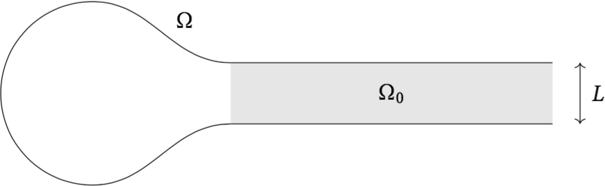
We assume that the round portion is sufficiently large that . Then, by Theorem 1, we know that (6) admits at least one solution. We can show that . Thus Theorem 3 applies when . The critical case is not covered by our result. Nonetheless, in [6 H. Berestycki and C. Graham, The steady states of strong-KPP reactions in general domains, in preparation (2022) ], we exploit the explicit structure of to prove that the solution of (6) is still unique in this case. This supports Conjecture 2.
Robin type conditions
Other types of boundary conditions are of interest as well. We can consider the Robin problem
where is the unit outward normal vector field on the boundary and is a constant. More generally, one might consider a function that varies on .
Conjecture 4. In a uniformly smooth domain with of strong KPP-type, the solution of problem (8) is unique when it exists.
In our forthcoming work [6 H. Berestycki and C. Graham, The steady states of strong-KPP reactions in general domains, in preparation (2022) ], we establish an analogue of Theorem 3 in the Robin case. This requires a suitable notion of the generalized principal Robin eigenvalue.
General positive and other reaction terms
In [6 H. Berestycki and C. Graham, The steady states of strong-KPP reactions in general domains, in preparation (2022) ], we also consider the more general class of positive nonlinear terms . This class is defined by the conditions
In all of space , uniqueness holds in the more general positive case. Indeed, under conditions (9), is the unique solution of (6) when . For a proof, I refer the reader to the forthcoming book [7 H. Berestycki and F. Hamel, Reaction-diffusion equations and propagation phenomena, Springer (to appear) ]. The presence of boundary changes matters significantly. In fact, in a proper subset with Dirichlet or Robin boundary, solutions of (6) (or (8)) need not be unique. However, uniqueness holds under Neumann boundary conditions.
In a uniformly smooth domain with of positive type (9), the unique solution of the Neumann problem (8) with is .
This result is a generalization of one in my earlier work with Hamel and Nadirashvili [9 H. Berestycki, F. Hamel and N. Nadirashvili, The speed of propagation for KPP type problems. II. General domains. J. Amer. Math. Soc. 23, 1–34 (2010) ]. This form is due to Rossi [15 L. Rossi, Stability analysis for semilinear parabolic problems in general unbounded domains. J. Funct. Anal. 279, Article ID 108657 (2020) ]. It naturally calls for the following.
267*
Problem. Can the result of Theorem 5 be extended to locally smooth domains?
(B) A problem in geometric analysis
by Michael Struwe (Departement Mathematik, ETH Zürich, Switzerland)
The last 40 years have seen enormous progress in the application of variational methods to problems in geometric analysis, which in general are characterized by the possibility of “bubbling” and topological degeneration of sequences of approximate solutions obtained either by regularization of the problem, or as “Palais–Smale sequences” for the energy functional involved. In critical point theory therefore it is vital to understand the possible interaction of the problem at hand with its “cousins” that characterize the “bubbling”, in particular, when the sought-after critical points are of “mountain-pass” type.
As an example consider the (by now classical) “Nirenberg problem” of finding conformal metrics of prescribed Gauss curvature on the standard -sphere, which has given rise to sophisticated analytic approaches and deep insights into the interplay of analysis and geometry, but which still poses a challenge, even though many partial answers have been obtained.
Nirenberg’s problem
After the work of Berger [16 M. S. Berger, Riemannian structures of prescribed Gaussian curvature for compact 2-manifolds. J. Differential Geom. 5, 325–332 (1971) ] and Kazdan–Warner [19 J. L. Kazdan and F. W. Warner, Curvature functions for compact 2-manifolds. Ann. of Math. (2) 99, 14–47 (1974) ] on conformal metrics of prescribed Gauss curvature on closed Riemann surfaces, the particular case, proposed by Nirenberg, of finding conformal metrics on the sphere with its standard round metric having a given function as Gauss curvature has attracted the attention of geometric analysts.
In view of the equation
relating and , where is the Laplace–Beltrami operator in the metric , for given , we need to solve the nonlinear partial differential equation
The problem is variational. Indeed, introducing the Liouville energy
where is the area element in the metric and denotes the average, and setting
for , the standard Sobolev space of -functions on with square-integrable weak derivatives, solutions of (10) may be characterized as critical points of .
Via the Möbius group of conformal diffeomorphisms of the sphere, for any point the functional may be compared with the functional
where is replaced by the constant . Indeed, given any , any , letting be the stereographic projection from the point and letting be the standard dilation, we obtain the Möbius map
Letting , where we write for brevity, we then have
(see for instance [17 S.-Y. A. Chang and P. C. Yang, Prescribing Gaussian curvature on S2. Acta Math. 159, 215–259 (1987) , Proposition 2.1]) and thus
For large , it was shown by Chang–Yang [17 S.-Y. A. Chang and P. C. Yang, Prescribing Gaussian curvature on S2. Acta Math. 159, 215–259 (1987) ] that the first and second variation of at may be related to and , respectively. From this observation, they deduce the following existence result.
Suppose that is a smooth function satisfying the non-degeneracy condition
and the index count condition
Then there is a smooth solution to (10).
Interpretation
Condition (13) in Theorem 6 may be interpreted in terms of the “last Morse inequality” related to the variational integral (11), that is, in terms of an equation identifying the “topological degree” of the (contractible) set of admissible functions with the sum of the topological degrees of all critical points of , including the contributions of the degenerate variational problems related to the functionals , . With what we remarked above, the latter contribution is given by the left-hand side of (13). Thus, if that term is different from , there has to be a further contribution to the total topological degree of all critical points, then necessarily coming from a solution to (10).
Open problem
In [23 M. Struwe, A flow approach to Nirenberg’s problem. Duke Math. J. 128, 19–64 (2005) ] an example was given showing that condition (13) in Theorem 6 in general cannot be removed; thus, with the non-degeneracy condition (12), condition (13) is not only sufficient but also in general necessary for the existence of a solution to (10).
However, we are still lacking a precise characterization of all solutions of (10). In particular, we should be able to obtain the existence of multiple solutions in certain cases. A simple instance of such a case, where – hopefully – the problem is feasible, would be when the given function is symmetric with respect to reflection in a plane and is a Morse function similar to the example studied in [23 M. Struwe, A flow approach to Nirenberg’s problem. Duke Math. J. 128, 19–64 (2005) ] but satisfying the Chang–Yang condition (13).
268*
Problem. Let be the set of functions with
having a saddle point at the north pole , a minimum at the south pole , and precisely two maxima as critical points, all of which are non-degenerate and satisfy (12), and such that condition (13) holds. Find conditions for such that there is more than one solution of (10), and characterize the set of all solutions of (10) in the sense of Morse theory.
Of course, the question may easily be widened to a larger class of functions.
Related challenges
Note that Chang–Yang [17 S.-Y. A. Chang and P. C. Yang, Prescribing Gaussian curvature on S2. Acta Math. 159, 215–259 (1987) ] showed that when solutions of (10) never are relative minima of the energy .
The Nirenberg problem thus can be seen in the larger context of finding critical points of “mountain-pass” type for variational problems characterized by conformal invariance and “bubbling”. A classic instance of such problems is in -dimensional gauge theory, in particular, in the question concerning the existence of -equivariant, non-minimal Yang–Mills connections in the trivial -bundle over , which remained open after Sibner–Sibner–Uhlenbeck [21 L. M. Sibner, R. J. Sibner and K. Uhlenbeck, Solutions to Yang–Mills equations that are not self-dual. Proc. Nat. Acad. Sci. U.S.A. 86, 8610–8613 (1989) ] obtained -equivariant, non-minimal Yang–Mills connections for any ; see also Donaldson [18 S. Donaldson, Karen Uhlenbeck and the calculus of variations. Notices Amer. Math. Soc. 66, 303–313 (2019) , pp. 309–310] for further details. Moreover, conformal invariance is responsible for many of the difficulties encountered by Rivière [20 T. Rivière, Willmore minmax surfaces and the cost of the sphere eversion. J. Eur. Math. Soc. (JEMS) 23, 349–423 (2021) ] in his recent work on “min-max” critical points for the Willmore energy related to sphere eversion.
Recall that Smale [22 S. Smale, A classification of immersions of the two-sphere. Trans. Amer. Math. Soc. 90, 281–290 (1958) ] famously showed that it is possible to “turn a sphere inside out” via a continuous path of -immersions of into . Moreover, Bryant characterized all immersed Willmore spheres in as being given by the images by inversions of simply connected, complete, non-compact minimal surfaces with planar ends, with Willmore energy given by , where is the number of ends, and index equal to . Finally, a topological result of Banchoff–Max shows that any path everting the sphere has to contain at least one immersion with a quadruple point and therefore, by a result of Li–Yau, with Willmore energy . Combining these pieces of information, Rivière conjectured that the inversion of a simply connected, complete minimal surface with planar ends, thus having index and Willmore energy , should give a “min-max Willmore sphere”, achieving the least maximal Willmore energy along paths of immersions of into that “turn the sphere inside out”. But in the variational ansatz “bubbling” may occur, and many questions remain to be solved. See [20 T. Rivière, Willmore minmax surfaces and the cost of the sphere eversion. J. Eur. Math. Soc. (JEMS) 23, 349–423 (2021) ] for further details and references.
Similarly, in gauge theory the desired -equivariant, non-minimal Yang–Mills connections in the trivial -bundle over should achieve the least maximal Yang–Mills energy along paths of connections beginning at a -equivariant Yang–Mills instanton and ending at a -equivariant anti-instanton. But again “bubbling” comes in the way.
III Solutions
252
Prove that the space of unordered couples of distinct points of a circle is the (open) Möbius band. More formally, consider
and the equivalence relation on this space ; prove that the quotient topological space is the (open) Möbius band. Costante Bellettini (Department of Mathematics, University College London, UK)
Solution by the proposer
The space of ordered pairs of points of a circle is the cartesian product , hence a torus. This is the same as the unit square with the following identifications: is identified with , both with orientation from left to right; is identified with , both with orientation from bottom to top. Note that the four vertices of the square are the same point. We now need to remove couples of the type (same point of the circle), which implicitly removes and as well. Hence, we are now looking at the square with the diagonal from to removed, and with and removed, keeping the identification we had earlier. Next, we need to identify couples and (since we want to study unordered couples). This amounts to removing one of the two triangles that have been obtained after removing the diagonal of the square; without loss of generality we assume that we remove the top-left triangle. What is left is the triangle with vertices , , , with the longer side removed (the one that was the diagonal of the square), with the point removed, and with the following identification: any point was identified (in the original torus) with the point , which has then been identified with the point . Hence, the triangle has the horizontal side oriented left-to-right identified with the vertical side oriented bottom-to-top. We can check that this is the (open) Möbius band as follows: the point is not in the triangle (nor is the longer side of the triangle), so we can stretch the point until the triangle becomes a rectangle, with the stretched point that has become the side opposite to the side that was the diagonal of the square. The identification of the remaining two sides gives the (open) Möbius band.
253
In the Euclidean plane, let and be two concentric circles of radius respectively and , with . Show that the locus of points such that the polar line of with respect to is tangent to is a circle of radius .
Acknowledgement
I want to thank the professors who guided me in the first part of my career for giving me the ideas for these problems.
Paola Bonacini (Mathematics and Computer Science Department, University of Catania, Italy)
Solution by the proposer
Let be any point such that the polar line of with respect to is tangent to . Then clearly is external to . Let be the centre of the two circles, and . Since is tangent to in , we can assert that the line is orthogonal to and, since is the polar of with respect to , the line is orthogonal to the line . So, the points , and are collinear and the angles , , and are right. We also know that , where . So we can assert that
and by looking at the triangle , we see that
Clearly, , and consequently,
This implies that
which clearly shows that is a circle of centre and radius .
254
Let be a connected open subset of Euclidean space, and suppose that the following conditions hold:
Every smooth irrotational vector field on admits a potential (i.e., it is the gradient of a smooth function).
The closure of is a smooth compact submanifold of (of course, with non-empty boundary).
Show that is simply connected. Does this conclusion hold even if we drop condition (2) on ? Roberto Frigerio (Dipartimento di Matematica, Università di Pisa, Italy)
Solution by the proposer
The usual scalar product on induces an identification between smooth vector fields and differential -forms, which identifies irrotational vector fields with closed forms, and fields admitting a potential with exact forms. Therefore, condition (1) may be restated as follows: every smooth -form on is exact, i.e., the first de Rham cohomology group of vanishes. By the de Rham Theorem, this is in turn equivalent to the fact that the singular homology module vanishes.
Since any compact manifold with boundary is homotopy equivalent to its interior, we may thus assume that . A well-known consequence of the Poincaré Duality Theorem is that, for any compact orientable -manifold with boundary , the dimension of is twice the dimension of . Since every codimension-0 submanifold of is obviously orientable, we thus have . Let be the components of the boundary . Since
and the -sphere is the only compact orientable -manifold without boundary with vanishing first cohomology group, we can conclude that is diffeomorphic to the -sphere for every .
It is well known that every smooth sphere in bounds asmooth closed disc (this is no longer true for non-smooth spheres; see below); hence, for every , we have , where is a smooth disc. Since is connected, it readily follows that there exists one of these closed discs, say , such that
In other words, is a closed disc with some open discs removed, and in particular it is simply connected.
In order to prove that is simply connected, the condition that be the interior of a compact smooth manifold with boundary is essential. Indeed, let be the well-known Alexander horned sphere. Then separates into two connected components: one of them, say , is homeomorphic to an open ball; the other one, say , is not simply connected. However, Alexander duality implies that
We thus have while . By setting , we thus get a non-simply connected open connected subset of such that every smooth irrotational vector field on admits a potential.
255
A regulus is a surface in that is formed as follows: We consider pairwise skew lines and take the union of all lines that intersect each of , , and . Prove that, for every regulus , there exists an irreducible polynomial of degree two that vanishes on . Adam Sheffer (Department of Mathematics, Baruch College, City University of New York, NY, USA)
Proof
Let be a set of 9 points that is obtained by arbitrarily choosing three points from each of , and . We write
Asking to vanish at a specific point is equivalent to a linear equation in the variables . Thus, asking to vanish at all points of yields a system of 9 linear equations with 10 variables. Since the number of variables is larger, this system admits a nontrivial solution. Thus, there exists a nonzero polynomial of degree at most two that vanishes on . Let be the set of points at which vanishes.
Let be the restriction of to the line . Since vanishes on at least three points of , the polynomial has at least three roots. Since but this polynomial has more than two roots, we have that . In other words, . By repeating the above argument, we get that . By definition, no plane contains a pair of skew lines, so cannot contain a plane. This implies that is irreducible of degree two.
Consider a line that intersects , and . Since these three lines are pairwise skew, the three intersection points are distinct, so . By restricting to as above, we get that . Since is the union of all such lines , we get that . This proof is by Larry Guth, although it may have also existed earlier.
256
(Enumerative Geometry). How many lines pass through generic lines in a -dimensional complex projective space ? Mohammad F. Tehrani (Department of Mathematics, University of Iowa, USA)
Introductory remarks
This is a problem in an over a century-old area of mathematics called enumerative geometry. Enumerative geometry is concerned with finding or counting geometric objects (mainly curves, i.e., -dimensional objects over the ground field) satisfying certain geometric conditions (e.g., passing through a specified set of objects or having a particular degree, genus, and types of singularities). Enumerative geometry was revolutionized in the mid-1990s by the novel predictions of mirror symmetry that led to the creation of Gromov–Witten theory and extensive study of such questions in complex algebraic geometry, symplectic geometry, and string-theoretic physics.
The most straightforward example in this area is the number of lines passing through two points, where the answer is . Here, one can interpret the word “line” as a real line in the real Euclidean space , a complex line in the complex Euclidean space , or a complex projective line (i.e., ) in the complex projective space . The answer is the same regardless of the context. The same is not true in most other questions. Gromov–Witten theory is mostly about counting complex curves in complex projective varieties or closed symplectic manifolds. The benefits of studying complex curves in compact complex/almost complex manifolds is two-fold. First, the compactness of the spaces involved results in finite counts. Second, working over complex numbers ensures that count of such objects does not depend on the choices involved. Recall that a degree- polynomial over has always roots (when counted with multiplicities), but a degree- polynomial over has at most roots.
Solution by the proposer
Before finding the answer, let us indeed argue that the expected answer is a finite number. As in linear algebra, this is done by computing degrees of freedom and the number of equations imposed by the constraints. As we mentioned above, there is exactly one line passing through two distinct points in ; the dimension of the space of pairs of such points is . However, for each line, there is a -dimensional family of pairs of points that yield that particular line. Therefore, assuming that the set of lines in is a nice geometric space, its dimension should be . The reduction in the dimension caused by the condition of intersecting any of the given lines is . It follows that the reduction in the dimension caused by the condition of intersecting all given four lines is . Since , the solution set should be discrete. Since we are working with compact spaces, it will indeed be finite. Bellow, using Schubert calculus on Grassmannians, we will compute this number. We challenge the reader to think about the following real affine version of the question using elementary techniques: How many lines pass through generic lines in ?
The -dimensional complex projective space is the projectivization of in the sense that each point in the former corresponds to a line in the latter. In one dimension higher, every projective line in is the projectivization of a plane in . Therefore, the space of lines in is the same as the space of planes in , which is known as the (complex) Grassmannian manifold . More generally, the Grassmannian is a compact complex -dimensional manifold that parametrizes the -dimensional subspaces of . Let be a line that is the projectivization of a two-dimensional subspace . The subspace of lines in that intersect is a submanifold of with . The points of correspond to two-dimensional subspaces such that . Even though depends on , the homology class of does not depend on . The homology groups of the Grassmannian are generated by a specific class of complex submanifolds known as Schubert cycles. All the odd degree homology groups are trivial.
Digression on Schubert calculus
Let be a sequence of non-negative integers between and , and define . Given a sequence of vector spaces , the Schubert cycle , with Poincaré dual , is defined to be
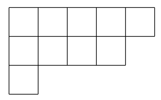
The homology class of does not depend on . There is a geometric way of describing a non-decreasing sequence which helps with understanding the computations involving Schubert cycles. A Young diagram is a finite collection of boxes, or cells, arranged in left-justified rows, with the row lengths weakly decreasing (each row has the same or shorter length than its predecessor). Listing the number of boxes in each row gives a sequence of non-negative integers, such that is the total number of boxes of the diagram. Figure 1 shows the Young diagram of . A special case of the so-called Pieri formula states that
where the left-hand side is the intersection of two cycles and the sum on the right-hand side is over all partitions which can be obtained by adding one box to the Young diagram of .
Going back to the counting of the proposed problem, it follows from (14) that . Therefore,
By Pieri’s formula, we have
Note that the Schubert cycle is the point (i.e., it generates ). It is straightforward (but crucial) to show that for generic lines , the intersection is transverse. We conclude that the answer to the proposed problem is .
257
I learned about the following problem from Shmuel Weinberger. It can be viewed as a topological analogue of Arrow’s Impossibility Theorem.
(a) A group of friends have decided to spend their summer cottaging together on an undeveloped island, which happens to be a perfect copy of the closed 2-disk . Their first task is to decide where on this island to build their cabin. Being democratically-minded, the friends decide to vote on the question. Each friend chooses his or her favourite point on . The friends want a function that will take as input their votes, and give as output a suitable point on to build. They believe, to be reasonable and fair, their “choice” function should have the following properties:
(Continuity) It should be continuous as a function . This means, if one friend changes their vote by a small amount, the output will change only a small amount.
(Symmetry) The friends should be indistinguishable from each other. If two friends swap votes, the final choice should be unaffected.
(Unanimity) If all friends chose the same point , then should be the final choice.
For which values of does such a choice function exist?
(b) The friends’ second task is to decide where along the shoreline of the island they will build their dock. The shoreline happens to be a perfect copy of the circle . Again, they decide to take the problem to a vote. For which values of does a continuous, symmetric, and unanimous choice function exist?
These are special cases of the following general problem in topological social choice theory: given a topological space , for what values of does admit a social choice function that is continuous, symmetric, and unanimous? In other words, when is there a function satisfying
is continuous,
is independent of the ordering of , and
for all ?
Jenny Wilson (Department of Mathematics, University of Michigan, USA)
Solution by the proposer
Consider the general problem described in the last paragraph. The statement that is independent of the ordering of is the statement that the function factors through the symmetric product, the quotient of by the action of the symmetric group , endowed with the quotient topology. Elements of are multisets of (not necessarily distinct) points in . The statement that is the statement that the composition
is the identity function. Thus the problem is equivalent to the following: does there exist a retraction from the symmetric product onto the image of the diagonal?
(a) An appropriate choice function exists for any . Identify the island (up to homeomorphism) with the closed unit disk in . Since the disk is convex, we can (for example) let
be the average value of the points.
(b) Such a choice function only exists for . We first consider the case , since this case reduces to a problem that will be familiar to many algebraic topology students.
The symmetric product is the Möbius band and the image of the diagonal is its boundary, as pictured.
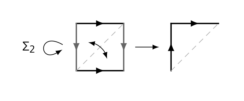
However, the boundary is not a retract of the Möbius band: the inclusion of the boundary induces the map on fundamental groups, which does not have a left inverse.
This argument generalizes for any . We can realize the -torus as the unit cube in with opposite faces identified. The corners are identified to a single point , which we choose as basepoint.
Let be a path from the origin to the point along mutually orthogonal edges of the cube, pictured here for . Construct (say, by straight-line homotopy) a based homotopy from the diagonal to .
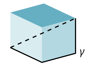
The orthogonal edges are identified in the symmetric product to a single loop. Thus, in the image of the diagonal (which equals the image of ) has an th root. The image of the diagonal in cannot be a retract.
For the general problem, Eckmann–Ganea–Hilton and later (independently) Weinberger proved the following results; see Eckmann’s survey [24 B. Eckmann, Social choice and topology: A case of pure and applied mathematics. Expo. Math. 22, 385–393 (2004) ].
Suppose that is homotopy equivalent to a finite simplicial complex. If is contractible, the function exists for any . If is not contractible, it exists only for .
Suppose that is homotopy equivalent to a connected CW complex. Then the map exists for all if and only if is a product of rational Eilenberg–MacLane spaces.
Weinberger [25 S. Weinberger, On the topological social choice model. J. Econom. Theory 115, 377–384 (2004) ] notes that there exist other infinite CW complexes for which a choice function exists for (some) arbitrarily large values of . For example, the infinite-dimensional real projective space admits a social choice function for any odd value of , but not for any even value.
We wait to receive your solutions to the proposed problems and ideas on the open problems. Send your solutions to Michael Th. Rassias by email to mthrassias@yahoo.com.
We also solicit your new problems with their solutions for the next “Solved and unsolved problems” column, which will be devoted to Number Theory.
References
- W. Malfliet and W. Hereman, The tanh method. I. Exact solutions of nonlinear evolution and wave equations. Phys. Scripta 54, 563–568 (1996)
- A.-M. Wazwaz, The tanh method for traveling wave solutions of nonlinear equations. Appl. Math. Comput. 154, 713–723 (2004)
- M. A. Xenos, An Euler–Lagrange approach for studying blood flow in an aneurysmal geometry. Proc. A. 473, 20160774 (2017)
- M. A. Xenos and A. C. Felias, Nonlinear dynamics of the KdV-B equation and its biomedical applications. In Nonlinear Analysis, Differential Equations, and Applications, Springer Optim. Appl. 173, Springer, Cham, 765–793 (2021)
- H. Berestycki, Le nombre de solutions de certains problèmes semi-linéaires elliptiques. J. Funct. Anal. 40, 1–29 (1981)
- H. Berestycki and C. Graham, The steady states of strong-KPP reactions in general domains, in preparation (2022)
- H. Berestycki and F. Hamel, Reaction-diffusion equations and propagation phenomena, Springer (to appear)
- H. Berestycki, F. Hamel and G. Nadin, Asymptotic spreading in heterogeneous diffusive excitable media. J. Funct. Anal. 255, 2146–2189 (2008)
- H. Berestycki, F. Hamel and N. Nadirashvili, The speed of propagation for KPP type problems. II. General domains. J. Amer. Math. Soc. 23, 1–34 (2010)
- H. Berestycki, F. Hamel and L. Rossi, Liouville-type results for semilinear elliptic equations in unbounded domains. Ann. Mat. Pura Appl. (4) 186, 469–507 (2007)
- H. Berestycki, L. Nirenberg and S. R. S. Varadhan, The principal eigenvalue and maximum principle for second-order elliptic operators in general domains. Comm. Pure Appl. Math. 47, 47–92 (1994)
- H. Berestycki and L. Rossi, Generalizations and properties of the principal eigenvalue of elliptic operators in unbounded domains. Comm. Pure Appl. Math. 68, 1014–1065 (2015)
- R. A. Fisher, The wave of advance of advantageous genes. Ann. Eugen. 7, 355–369 (1937)
- A. N. Kolmogorov, I. G. Petrovsky and N. S. Piskunov, Étude de l’équation de la diffusion avec croissance de la quantité de matière et son application à un problème biologique. Bull. Univ. Moskow, Ser. Internat., Sec. A 1, 1–25 (1937)
- L. Rossi, Stability analysis for semilinear parabolic problems in general unbounded domains. J. Funct. Anal. 279, Article ID 108657 (2020)
- M. S. Berger, Riemannian structures of prescribed Gaussian curvature for compact 2-manifolds. J. Differential Geom. 5, 325–332 (1971)
- S.-Y. A. Chang and P. C. Yang, Prescribing Gaussian curvature on S2. Acta Math. 159, 215–259 (1987)
- S. Donaldson, Karen Uhlenbeck and the calculus of variations. Notices Amer. Math. Soc. 66, 303–313 (2019)
- J. L. Kazdan and F. W. Warner, Curvature functions for compact 2-manifolds. Ann. of Math. (2) 99, 14–47 (1974)
- T. Rivière, Willmore minmax surfaces and the cost of the sphere eversion. J. Eur. Math. Soc. (JEMS) 23, 349–423 (2021)
- L. M. Sibner, R. J. Sibner and K. Uhlenbeck, Solutions to Yang–Mills equations that are not self-dual. Proc. Nat. Acad. Sci. U.S.A. 86, 8610–8613 (1989)
- S. Smale, A classification of immersions of the two-sphere. Trans. Amer. Math. Soc. 90, 281–290 (1958)
- M. Struwe, A flow approach to Nirenberg’s problem. Duke Math. J. 128, 19–64 (2005)
- B. Eckmann, Social choice and topology: A case of pure and applied mathematics. Expo. Math. 22, 385–393 (2004)
- S. Weinberger, On the topological social choice model. J. Econom. Theory 115, 377–384 (2004)
Cite this article
Michael Th. Rassias, Solved and unsolved problems. Eur. Math. Soc. Mag. 125 (2022), pp. 53–62
DOI 10.4171/MAG/103