
1 Introduction
Tensors networks are ubiquitous in most areas of modern science including data science [11 A. Cichocki, Tensor networks for big data analytics and large-scale optimization problems, preprint, arXiv:1407.3124 (2014) ], condensed matter physics [19 C. Fernández-González, N. Schuch, M. M. Wolf, J. I. Cirac and D. Pérez-García, Frustration free gapless Hamiltonians for matrix product states. Comm. Math. Phys. 333, 299–333 (2015) ], string theory [22 A. Jahn and J. Eisert, Holographic tensor network models and quantum error correction: A topical review. Quantum Sci. Technol. 6, 033002 (2021) ] and quantum computer science. The manners in which tensors are employed/treated exhibit significant overlap across many of these areas. In data science, tensors are used to represent large datasets. In condensed matter physics and in quantum computer science, tensors are used to represent states of quantum systems.
Manipulating large tensors comes at a high computational cost [28 A. Novikov, D. Podoprikhin, A. Osokin and D. P. Vetrov, Tensorizing neural networks. Adv. Neural Inf. Process. Syst. 28 (2015) ]. This observation has inspired techniques for tensor decompositions that would reduce computational complexity while preserving the original data that they represents. Such techniques are now known as tensor network methods.
Tensor networks have risen to prominence in the last fifteen years, with several European schools playing leading roles in their modern development, as a means to describe and approximate quantum states (see the review [14 J. I. Cirac, D. Pérez-García, N. Schuch and F. Verstraete, Matrix product states and projected entangled pair states: Concepts, symmetries, theorems. Rev. Modern Phys. 93, 045003 (2021) ]). The topic however dates back much further, to work of Penrose [32 R. Penrose, Applications of negative dimensional tensors. In Combinatorial Mathematics and its Applications (Proc. Conf., Oxford, 1969), Academic Press, London, 221–244 (1971) ] and in retrospect, even arose as special cases in work of Cayley [10 A. Cayley, On the theory of groups as depending on the symbolic equation θn=1. Philos. Mag. 7, 40–47 (1854) ]. Tensor networks have a rich modern history in mathematical physics [32 R. Penrose, Applications of negative dimensional tensors. In Combinatorial Mathematics and its Applications (Proc. Conf., Oxford, 1969), Academic Press, London, 221–244 (1971) ], in category theory [44 P. Selinger, A survey of graphical languages for monoidal categories. In New Structures for Physics, Lecture Notes in Phys. 813, Springer, Heidelberg, 289–355 (2011) ], in computer science, algebraic logic and related disciplines [1 J. Baez and M. Stay, Physics, topology, logic and computation: A Rosetta Stone. In New Structures for Physics, Lecture Notes in Phys. 813, Springer, Heidelberg, 95–172 (2011) ]. Such techniques are now becoming more common in data science and machine learning (see the reviews [12 A. Cichocki, N. Lee, I. Oseledets, A.-H. Phan, Q. Zhao and D. P. Mandic, Tensor networks for dimensionality reduction and large-scale optimization. I: Low-rank tensor decompositions. Found. Trends Mach. Learn. 9, 249–429 (2016) , 13 A. Cichocki, A.-H. Phan, Q. Zhao, N. Lee, I. Oseledets, M. Sugiyama and D. P. Mandic, Tensor networks for dimensionality reduction and large-scale optimization. II: Applications and future perspectives. Found. Trends Mach. Learn. 9, 431–673 (2017) ]).
1.1 Basic material about multilinear maps
It might be stated that the objective of linear algebra is to classify linear operators up to isomorphism and study the simplest representative in each equivalence class. This motivates the prevalence of decompositions such as SVD, LU and the Jordan normal form. A special case of linear operators are linear maps from a vector space to an arbitrary field like or . These linear maps form the dual space (vector space of covectors) to our vector space .
A natural generalisation of linear maps is provided by the multilinear maps, i.e., maps that are linear in each argument when the values of other arguments are fixed. For a given pair of non-negative integers and , a type- tensor is defined as a multilinear map
where is an arbitrary field. The tensor is said to be of order (valence) . Note that some authors refer to this as rank , but we will never do that.
It is often more convenient to view tensors as elements of a vector space known as the tensor product space. Thus, the above -tensor in this alternative interpretation can be defined as an element
Moreover, the universality property of tensor products of vector spaces states that any multilinear map can be replaced by a unique linear map acting from the tensor product of vector spaces to the base field.
If we assume the axiom of choice, every vector space admits a Hamel basis. If is such a basis in , then the components of a tensor are therefore the coefficients of with respect to the basis and its dual basis (basis of the dual space ), that is
Adopting Einstein’s summation convention, summation over repeated indices is implied in (2).
Returning to (1), given covectors and vectors , the value of the tensor is evaluated as
where and are numbers obtained by evaluating covectors (functionals) at the corresponding vectors. In quantum computation, the basis vectors are denoted by and the basis covectors are denoted by . Using Dirac’s notation, tensor products are written in compact form as
and the tensor takes the form
Similarly, given a tuple of covectors and vectors we write them as and , as elements of the corresponding tensor product space(s).
In this notation the evaluation (3) takes the form
Since in quantum computation the vector spaces under consideration as well as their duals are Hilbert spaces, Riesz’s representation theorem for linear functionals implies that the evaluation above can be seen as an inner product.
Finally, a tensor can be identified with the array of coefficients in a specific basis decomposition. This approach is not basis independent, but is useful in applications. Henceforth in this review we will fix the standard basis, which will establish a canonical isomorphism between the vector space and its dual. In the simplest case , for example, this gives us the following equivalences:
In the more general case this leads to the equivalence between the components and . Given a valence- tensor , the total number of tensors in the equivalence class formed by raising, lowering and exchanging indices has cardinality (see [4 J. Biamonte and V. Bergholm, Tensor networks in a nutshell, preprint, arXiv:1708.00006 (2017) ]). Recognising this arbitrariness, Penrose considered a graphical depiction of tensors [32 R. Penrose, Applications of negative dimensional tensors. In Combinatorial Mathematics and its Applications (Proc. Conf., Oxford, 1969), Academic Press, London, 221–244 (1971) ], stating that “it now ceases to be important to maintain a distinction between upper and lower indices.” This convention is widely adopted in the contemporary literature.
1.2 Tensor trains aka matrix product states
Consider a tensor with components with . Hence, has components, a number that can exceed the total number of electrons in the universe when is as small as and . Clearly, storing the components of such a large tensor in a computer memory and subsequently manipulating it can become impossible. The good news is that for most practical purposes, a tensor typically contains a large amount of redundant information. This enables factoring of into a sequence of “smaller” tensors.
Tensor trains (see [31 I. V. Oseledets, Tensor-train decomposition. SIAM J. Sci. Comput. 33, 2295–2317 (2011) ]) and matrix product states (MPS) [33 D. Perez-Garcia, F. Verstraete, M. M. Wolf and J. I. Cirac, Matrix product state representations. Quantum Inf. Comput. 7, 401–430 (2007) , 30 R. Orús, Advances on tensor network theory: Symmetries, fermions, entanglement, and holography. Eur. Phys. J. B 87, 280 (2014) ] arose in data science and in condensed matter physics, where it was shown that any tensor with components admits a decomposition of the form
where is an -dimensional matrix, and and as - and -dimensional vectors, respectively.
Likewise, an -qubit state , written in the computational basis as , , can equivalently be expressed as
Here is a dimensional matrix and are and dimensional vectors, respectively. Note that here we are adhering to the braket notation, as is customary in quantum mechanics. The representation of in (5) is called the matrix product state representation with an open boundary condition (OBC-MPS). See Figure 1 for a graphical representation.

Yet another useful MPS decomposition that a state might admit is the MPS with periodic boundary condition (PBC-MPS) [30 R. Orús, Advances on tensor network theory: Symmetries, fermions, entanglement, and holography. Eur. Phys. J. B 87, 280 (2014) ]. The PBC-MPS representation of an -qubit state
is given by
where is an matrix. The graphical representation of a PBC-MPS is shown in Figure 2.

An -qubit state has independent coefficients . The MPS representation of , on the other hand, is less data intensive. If is an matrix for all , the size of the representation becomes , which is linear in for a constant . The point of the method is to choose such that a good and compact approximation of is obtained. The number is often also referred to as the virtual bond dimension. Data compression becomes even more effective if the MPS is site independent, that is, if for all . It has been shown that a site-independent representation of a PBC-MPS always exists if the state is translation invariant [33 D. Perez-Garcia, F. Verstraete, M. M. Wolf and J. I. Cirac, Matrix product state representations. Quantum Inf. Comput. 7, 401–430 (2007) ]. Note that MPS is invariant under the transformation for any invertible ; this follows from the cyclicity of the trace operator. Therefore, it is often customary to impose an additional constraint here, viz. , in order to fix the gauge freedom [14 J. I. Cirac, D. Pérez-García, N. Schuch and F. Verstraete, Matrix product states and projected entangled pair states: Concepts, symmetries, theorems. Rev. Modern Phys. 93, 045003 (2021) ] (see also the connections to algebraic invariant theory [5 J. Biamonte, V. Bergholm and M. Lanzagorta, Tensor network methods for invariant theory. J. Phys. A 46, 475301 (2013) ]).
2 Machine learning: classical to quantum
2.1 Classical machine learning
At the core of machine learning is the task of data classification. In this task, we are typically provided with a labelled dataset , where the vectors are the input data (e.g., animal images) and the vectors are the corresponding labels (e.g., animal types). The objective is to find a suitable machine learning model with tunable parameters that generates the correct label for a given input . Note that our model can be looked upon as a family of functions parameterised by : takes a data vector as an input and outputs a predicted label; for an input datum , the predicted label is . To ensure that our model generates the correct labels, it needs to be trained; in order to accomplish this, a training set is chosen, the elements of which serve as input data to train . Training requires a cost function,
where measures the mismatch between the real label and the estimated label. Typical choices for include, e.g., the negative log-likelihood function, mean squared errors (MSE), etc. [37 L. Rosasco, E. De Vito, A. Caponnetto, M. Piana and A. Verri, Are loss functions all the same? Neural Comput. 16, 1063–1076 (2004) ]. By minimising (7) with respect to , one obtains the value , which completes the training. After the model has been trained, we can evaluate its performance by feeding it inputs from (often referred to as the validation set) and checking for classification accuracy.
For a more formal description, let us assume that the dataset is sampled from a joint probability distribution with a density function . The role of a classifier model is to approximate the conditional distribution . The knowledge of allows us, in principle, to establish theoretical bounds on the performance of the classifier. Consider the generalisation error (also called risk), defined as . A learning algorithm is said to generalise if ; here is the cardinality of the training set. However, since in general we do not have access to we can only attempt to provide necessary conditions to bound the difference of the generalisation error and the empirical error by checking certain stability conditions to ensure that our learning model is not too sensitive to noise in the data [8 O. Bousquet and A. Elisseeff, Stability and generalization. J. Mach. Learn. Res. 2, 499–526 (2002) ]. For example, we can try to ensure that our learning model is not affected if one of the data points is left out during training. The technique of regularisation prevents overfitting.
Several different types of machine learning models exist, which range from fairly elementary models, such as perceptrons, to highly involved ones, such as deep neural networks (DNNs) [24 Y. LeCun, Y. Bengio and G. Hinton, Deep learning. Nature 521, 436–444 (2015) , 38 F. Rosenblatt, The perceptron: A probabilistic model for information storage and organization in the brain. Psychol. Rev. 65, 386 (1958) ]. The choice of is heavily dependent on the classification task, the type of the dataset, and the desired training properties. Consider a dataset with two classes (a binary dataset) that is linearly separable. That is, (i) and (ii) one can construct a hyperplane that separates the input data belonging to the different classes. Finding this hyperplane, aka the decision boundary, is therefore sufficient for data classification in . This task can be accomplished with a simplistic machine learning model—the perceptron—which is in fact a single McCulloch–Pitts neuron [26 W. S. McCulloch and W. Pitts, A logical calculus of the ideas immanent in nervous activity. Bull. Math. Biophys. 5, 115–133 (1943) ]. The algorithm starts with the candidate solution for the hyperplane , where are tunable parameters and play the role of . It is known from the perceptron convergence algorithm that one can always find a set of parameters , such that for every , if , then , while if , then .
Most datasets of practical importance, however, are not linearly separable and consequently cannot be classified by the perceptron model alone. Assuming that is a binary dataset which is not linearly separable, we consider a map , , with the proviso that is nonlinear in the components of its inputs [6 C. M. Bishop, Pattern recognition and machine learning. Information Science and Statistics, Springer, New York (2006) ]. In machine learning is called a feature map and the vector space is known as a feature space. Thus nonlinearly maps each input datum to a vector in the feature space. The significance of this step follows from Cover’s theorem on separability of patterns [16 T. M. Cover, Geometrical and statistical properties of systems of linear inequalities with applications in pattern recognition. IEEE Trans. Electron. Comput. 14, 326–334 (1965) ], which suggest that the transformed dataset is more likely to be linearly separable. For a good choice of , the data classification step now becomes straightforward, as it is sufficient to fit a hyperplane to separate the two classes in the feature space. Indeed, the sought-for hyperplane can be constructed, using the perceptron model, provided the feature map is explicitly known. Actually, a hyperplane can still be constructed even when is not explicitly known. A particularly elegant way to accomplish this is via the support vector machine (SVM) [15 C. Cortes and V. Vapnik, Support-vector networks. Mach. Learn. 20, 273–297 (1995) ], by employing the so-called kernel trick [45 J. Shawe-Taylor, N. Cristianini et al., Kernel methods for pattern analysis. Cambridge University Press, Cambridge (2004) ].
Consider again the binary dataset . The aim is to construct a hyperplane that separates the samples belonging to the two classes. In addition, we would like to maximise the margin of separation. Formally, we search for a set of parameters such that for every , if , then , while if , then . As in the perceptron model, the SVM algorithm starts with the candidate solution and the parameters are tuned based on the training data. An interesting aspect of the SVM approach, however, is the dependence of the algorithm on a special subset of the training data called support vectors, namely, the ones that satisfy the relation . We assume that there are such vectors , . With some algebra, which we omit here, it can be shown that the decision boundary is given by the hyperplane
where
with the additional conditions and . All summations in (10) are over the entire training set. We make a key observation here: from (8), (9) and (10) we see that the expression of the decision boundary has no explicit dependence on the feature vectors . Instead, the dependence is solely on the inner products of the form . This allows us to use the kernel trick.
Support functions in optimisation
If is a nonempty closed convex set, the support function of is given by . The hyperplane is called a supporting hyperplane of with outer unit normal vector . The function outputs the signed distance of from the origin. The data points that lie on are called support vectors in the machine learning literature.
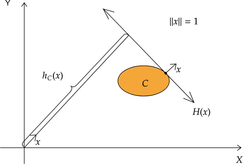
Graphical representation of the support function and supporting hyperplane.
Kernel functions
The concept of the kernel function originates in the theory of Reproducing Kernel Hilbert Spaces (RKHS). Consider a Hilbert space consisting of real-valued functions defined on an arbitrary set . We can define an evaluation functional that maps each function to a real number. If for every the linear functional is bounded on we call an RKHS. Applying Riesz’s theorem mentioned in the introduction, we have the representation , where . It follows that .
The function is called the reproducing kernel of the space . Briefly, in an RKHS the evaluation of a function at a point can be replaced by taking an inner product with a function determined by the kernel in the associated function space.
Now given a feature map , where is a Hilbert space, we define a normed space with the norm . One can show that is a RKHS with the kernel .
Formally, a kernel is defined as a function that computes the inner product of the images of in the feature space, i.e., . Accordingly, all the inner products in (8), (9) and (10) can be replaced by the corresponding kernels. We can then use the kernel trick, that is, assign an analytic expression for the kernel in (8), (9) and (10), provided that the expression satisfies all the required conditions for it to be an actual kernel [39 B. Schölkopf, A. J. Smola, F. Bach et al., Learning with kernels: Support vector machines, regularization, optimization, and beyond. MIT Press (2002) ]. Indeed, every choice of a kernel can be implicitly associated to a feature map . However, in the current approach we do not need to know the explicit form of the feature map. In fact, this is the advantage of the kernel trick, as calculating is less efficient than using the kernels directly.
Most modern applications in machine learning, however, involve deep neural networks (DNNs) [43 H. Schulz and S. Behnke, Deep learning. KI-Künstliche Intelligenz 26, 357–363 (2012) ]. A DNN can also be regarded as a collection of perceptrons arranged in a definite fashion. The architecture of a DNN is best understood and visualised in the form of a graph. Specifically, a DNN is composed of an input layer, an output layer, and several intermediate hidden layers. Each layer consists of several nodes. Each of these nodes represents a neuron. Edges are allowed to exist between nodes belonging to adjacent layers only: nodes in layer share edges with nodes in layer and nodes in layer . For the sake of simplicity, we consider the case where all the nodes in the -th layer are connected to all the nodes in the -th layers—a fully connected neural network.
A DNN takes a data vector as an input (at the input layer). This input is subsequently manipulated by the neurons in the next layer (the first hidden layer) to output a transformed vector , and this process is repeated till the last layer (output layer) is reached. Consider the -th neuron in the -th layer; for convenience, we denote this neuron by . It receives an input vector whose components are the outputs of the neurons in the -th layer, and then transforms by the rule
where are weights associated with the edges that connect the neuron to the neurons in the previous layer, is the bias corresponding to the neuron , and is a differentiable nonlinear function known as the activation function. This is the fundamental mathematical operation that propagates data in a DNN, layer by layer, in the forward direction (input layer to output layer), through a series of complex transformations. The training component of the algorithm is however accomplished through the back-propagation step [35 R. Rojas, The backpropagation algorithm. In Neural Networks, Springer, 149–182 (1996) ]: a cost function is calculated by comparing the signal at the output layer (the model predicted label for the data ) and the desired signal (the actual label for the data ), based on which the weights and the biases are adjusted so that the cost function is minimised. Apart from supervised learning, DNNs are routinely used for unsupervised learning, including generative learning. In generative learning, given access to a training dataset, a machine learning model learns its underlying probability distribution for future sample generation. To formulate this mathematically, consider a dataset , whose entries are independent and identically distributed vectors and are sampled according to a distribution . The purpose of a generative model is to approximate , given the access to training data from the dataset . To achieve this, a machine learning model (with tunable parameters ) is trained so that the model generated distribution, , mimics the true distribution. The standard practice in generative learning is to minimise the negative log-likelihood with respect to the model parameters, which is tantamount to minimising the Kullback–Leibler divergence between the two distributions.
2.2 Variational algorithms and quantum machine learning (QML)
Variational quantum computing has emerged as the preeminent model for quantum computation. The model merges ideas from machine learning to better utilise modern quantum hardware.
Mathematically, the problem in variational quantum computing can be formulated as follows: given (i) a variational quantum circuit (aka ansatz) which produces an -qubit variational state ; , (ii) an objective function , and (iii) the expectation , find
Then will approximate the ground state (eigenvector corresponding to the lowest eigenvalue) of the Hamiltonian . The operator , often called the problem Hamiltonian, can suitably treat several classes of problems so that the solution to a problem is encoded in the ground state of . The variational model of quantum computation was shown to be universal in [3 J. Biamonte, Universal variational quantum computation. Phys. Rev. A 103, L030401 (2021) ].
Quantum machine learning, both discriminative and generative, emerged as an important application of variational algorithms with suitable modifications to the aforementioned scheme. Indeed, by their very design, variational algorithms are well suited to implement machine learning tasks on a quantum device. The earlier developments in QML came mainly in the form of classification tasks [27 K. Mitarai, M. Negoro, M. Kitagawa and K. Fujii, Quantum circuit learning. Phys. Rev. A 98, 032309 (2018) , 18 E. Farhi and H. Neven, Classification with quantum neural networks on near term processors, preprint, arXiv:1802.06002 (2018) ].
Classification of a classical dataset on quantum hardware typically involves four steps. First, the input vector is embedded into an -qubit state . The effect of data encoding schemes on the expressive power of a quantum machine learning model was studied in [42 M. Schuld, R. Sweke and J. J. Meyer, Effect of data encoding on the expressive power of variational quantum-machine-learning models. Phys. Rev. A 103, 032430 (2021) ]. What is the most effective data embedding scheme? Although there are several interesting candidates [25 S. Lloyd, M. Schuld, A. Ijaz, J. Izaac and N. Killoran, Quantum embeddings for machine learning, preprint, arXiv:2001.03622 (2020) , 34 A. Pérez-Salinas, A. Cervera-Lierta, E. Gil-Fuster and J. I. Latorre, Data re-uploading for a universal quantum classifier. Quantum 4, 226 (2020) ], this question remains largely unanswered. In the second step, a parameterised ansatz is applied to to output . A number of different ansatzes are in use today, including the hardware efficient ansatz, the checkerboard ansatz, the tree tensor network ansatz, etc., which are chosen according to the application and implementation specifications under consideration. The third step in the process is where data is read out of : expectation values of certain chosen observables (Hermitian operators) are calculated with respect to to generate a predicted label . The measured operators are typically the Pauli strings, which form a basis in . In the final step, a cost function is constructed as in (7) and minimised by tuning . This approach was used in several studies to produce successful classifications in practical datasets (see, e.g., [40 M. Schuld, A. Bocharov, K. M. Svore and N. Wiebe, Circuit-centric quantum classifiers. Phys. Rev. A 101, 032308 (2020) ]).
An interesting variation of the approach described above was shown in [41 M. Schuld and N. Killoran, Quantum machine learning in feature Hilbert spaces. Phys. Rev. Lett. 122, 040504 (2019) , 21 V. Havlíček, A. D. Córcoles, K. Temme, A. W. Harrow, A. Kandala, J. M. Chow and J. M. Gambetta, Supervised learning with quantum-enhanced feature spaces. Nature 567, 209–212 (2019) ] to implement data classification based on the kernel trick. In this method the Hilbert space is treated as a feature space and the data embedding step, , as a feature map. A quantum circuit is used directly to compute the inner product , using, e.g., the swap test, which is then employed for data classification by means of classical algorithms such as SVMs.
Quantum machine learning has also been used to classify genuine quantum data. Some prominent examples of such applications include: classifying phases of matter [47 A. V. Uvarov, A. S. Kardashin and J. D. Biamonte, Machine learning phase transitions with a quantum processor. Phys. Rev. A 102, 012415 (2020) ], quantum channel discrimination [23 A. Kardashin, A. Pervishko, D. Yudin, J. Biamonte et al., Quantum machine learning channel discrimination, preprint, arXiv:2206.09933 (2022) ], and entanglement classification [20 E. Grant, M. Benedetti, S. Cao, A. Hallam, J. Lockhart, V. Stojevic, A. G. Green and S. Severini, Hierarchical quantum classifiers. npj Quantum Inf. 4, 1–8 (2018) ]. Other machine learning problems with quantum mechanical origins that have been solved by variational algorithms include quantum data compression [36 J. Romero, J. P. Olson and A. Aspuru-Guzik, Quantum autoencoders for efficient compression of quantum data. Quantum Sci. Technol. 2, 045001 (2017) ] and denoising of quantum data [7 D. Bondarenko and P. Feldmann, Quantum autoencoders to denoise quantum data. Phys. Rev. Lett. 124, 130502 (2020) ]. Both of these applications use a quantum autoencoder. A quantum autoencoder, much like its classical counterparts, consists of two parts: an encoder and a decoder. The encoder removes the redundant information from the input data to produce a minimal low-dimensional representation. This process is known as feature extraction. To ensure that the minimal representation produced by the encoder is efficient, a decoder is used which takes the output of the encoder and tries to reconstruct the original data. Thus, in an autoencoder, both the encoder and the decoder are trained in tandem to ensure that the input at the encoder and the output at the decoder closely match each other. While in the classical case the encoders and the decoders are chosen to be neural networks, in the quantum version of an autoencoder neural networks are replaced by variational circuits.
Considerable advances were made on the front of quantum generative learning as well. In [2 M. Benedetti, D. Garcia-Pintos, O. Perdomo, V. Leyton-Ortega, Y. Nam and A. Perdomo-Ortiz, A generative modeling approach for benchmarking and training shallow quantum circuits. npj Quantum Inf. 5, 1–9 (2019) ] it was shown that generative modelling can be used to prepare quantum states by training shallow quantum circuits. The central idea is to obtain the model generated probability distribution by performing repeated measurements on a variational state . The state is prepared on a short-depth circuit with a fixed ansatz and parameterised with the vector . The target distribution is also constructed in much the same manner, by performing repeated measurements on the target state. The measurement basis (preferably informationally complete positive operator-valued measures), as expected, is kept to be the same in both cases. The training objective therefore is to ensure that mimics so that the variational circuit learns to prepare the target state. The same task in an alternate version can be looked upon as a machine-learning assisted quantum state tomography [9 J. Carrasquilla, G. Torlai, R. G. Melko and L. Aolita, Reconstructing quantum states with generative models. Nat. Mach. Intell. 1, 155–161 (2019) ].
3 Tensor networks in machine learning
3.1 Tensor networks in classical machine learning
Recently tensor network methods have found several applications in machine learning. Here we discuss some of these applications with a focus on supervised learning models. We return to our labelled dataset , where . As mentioned earlier, there are several machine learning models to choose from to perform a classification on the dataset .
However, in more abstract terms, a classifier can be expressed as a function of the form
in the polynomial basis [29 A. Novikov, M. Trofimov and I. Oseledets, Exponential machines, preprint, arXiv:1605.03795 (2016) ]. Here is an input datum and is the -th component of . The tensor is what we call as the weight tensor, which encodes the tunable parameters in . Going back to the case of binary classification, that is, , can be regarded as a surface in that can be tuned (trained) so that it acts as a decision boundary between the two classes of input data. Indeed, the training can be accomplished by the minimisation
where is the predicted label. However, in practice we run into a bottleneck when we compute (12), since this involves components of the weight tensor. One way to circumvent this bottleneck is to express the weight tensor as a MPS. Following the observation in Section 1.2, for a suitable choice of the virtual bond dimension , the MPS representation of the weight tensor would involve only components, thus making the computation of (12) less resource intensive [46 E. Stoudenmire and D. J. Schwab, Supervised learning with tensor networks. Adv. Neural Inf. Process. Syst. 29 (2016) ]. Here it is worth noting that we could alternatively have opted for any other basis in the decomposition of the function , depending on the optimisation problem at hand.
Yet another application of tensor networks in machine learning can be seen in DNNs. Consider the transformation in (11). For most practically relevant DNNs, this transformation is highly resource intensive. This is due to the fact that the vectors are typically very large and hence computing the inner products is difficult. This computation can be made efficient by using MPS. In order to do this, the vectors are first reshaped, converting them into tensors and then expressing them as an MPS. When we express a vector as a MPS we need to keep track of much fewer components compared to the original representation. This makes the computation of (11) tractable.
3.2 The parent Hamiltonian problem
Consider the quantum state preparation problem using a variational algorithm. Given a variational circuit and an -qubit target state , tune such that approximates . To accomplish this task one needs to construct a Hamiltonian with as its unique ground state, which will serve as the objective function of the algorithm. Constructing such a Hamiltonian for a given target state is known as the parent Hamiltonian problem. The simplest recipe is to set . This construction is however not always useful, because expressing in the basis of Pauli strings—the basis of measurement—may require an exponential number of terms. Thus estimating the expectation of in polynomial time becomes unfeasible.
Ideally, we want the sought-for Hamiltonian to enjoy the following properties:
The Hamiltonian is non-negative.
The Hamiltonian has a non-degenerate (unique) ground state .
The Hamiltonian is gapped. An -qubit Hamiltonian is said to be gapped if
Validity of (13) ensures that is gapped for all finite .
The Hamiltonian is local. An -qubit Hamiltonian is said to be local if it can be expressed as
where is the set of symbols (qubits) and , where . The Hamiltonian is said to be -local if none of the ’s operates on more than symbols (qubits) nontrivially; here a trivial operation refers to the case when is the identity for some index .
The Hamiltonian must have terms when expressed in the Pauli basis. The number of terms in a Hamiltonian when expressed in the Pauli basis is also known as the cardinality of the Hamiltonian, (see [3 J. Biamonte, Universal variational quantum computation. Phys. Rev. A 103, L030401 (2021) ]).
Hamitonians with such properties can indeed be constructed if admits a matrix product state, albeit with the additional requirement that must satisfy the injectivity condition. For the parent Hamiltonian construction consider the following setting. Let be an -qubit state written as a translation-invariant and site-independent MPS with periodic boundary conditions:
where . For the sake of brevity we will call these matrices Kraus operators.1There is indeed there a connection between the matrices and completely positive trace-preserving (CPTP) maps from which the derive their name. For the purpose of this paper, however, we will skip the detailed explanation. Consider the map
where . We say that the state is injective with injectivity length if the map is injective. Several corollaries follow from this definition. A particularly useful one connects the notion of injectivity to the rank of reduced density matrices. It asserts that for an -qubit reduced density matrix, , of , we have if injectivity holds. It has been shown that in the large- limit, is given by
with , and . Alternatively, this would mean that is a linearly independent set.
The form of the reduced density matrix in (14) is particularly telling and allows us to construct the parent Hamiltonian of : . We formally write our parent Hamiltonian as
where operates nontrivially over -qubits from to and obeys the condition . The latter condition combined with (14) ensures that for all , which in turn implies that . In fact, , provided is injective, and so condition 1 for is satisfied. Conditions 3 and 4 are satisfied naturally due to the form of in (15). In addition, can also seen to be frustration free, that is, for all . Finally, it was shown in [17 M. Fannes, B. Nachtergaele and R. F. Werner, Finitely correlated states on quantum spin chains. Comm. Math. Phys. 144, 443–490 (1992) ] that if is injective, then is gapped.
4 Conclusion
The importance of matrix product states in physics is due to the ease with which one could calculate and verify important quantities or properties, such as two-point functions, thermal properties, and more. This is also true in machine learning applications. For example, images of size can be viewed as rank-one tensor networks on . Departing from this linear (train) structure results in tensors with potentially much greater expressability at the cost of many desirable properties being lost.
- 1
There is indeed there a connection between the matrices and completely positive trace-preserving (CPTP) maps from which the derive their name. For the purpose of this paper, however, we will skip the detailed explanation.
References
- J. Baez and M. Stay, Physics, topology, logic and computation: A Rosetta Stone. In New Structures for Physics, Lecture Notes in Phys. 813, Springer, Heidelberg, 95–172 (2011)
- M. Benedetti, D. Garcia-Pintos, O. Perdomo, V. Leyton-Ortega, Y. Nam and A. Perdomo-Ortiz, A generative modeling approach for benchmarking and training shallow quantum circuits. npj Quantum Inf. 5, 1–9 (2019)
- J. Biamonte, Universal variational quantum computation. Phys. Rev. A 103, L030401 (2021)
- J. Biamonte and V. Bergholm, Tensor networks in a nutshell, preprint, arXiv:1708.00006 (2017)
- J. Biamonte, V. Bergholm and M. Lanzagorta, Tensor network methods for invariant theory. J. Phys. A 46, 475301 (2013)
- C. M. Bishop, Pattern recognition and machine learning. Information Science and Statistics, Springer, New York (2006)
- D. Bondarenko and P. Feldmann, Quantum autoencoders to denoise quantum data. Phys. Rev. Lett. 124, 130502 (2020)
- O. Bousquet and A. Elisseeff, Stability and generalization. J. Mach. Learn. Res. 2, 499–526 (2002)
- J. Carrasquilla, G. Torlai, R. G. Melko and L. Aolita, Reconstructing quantum states with generative models. Nat. Mach. Intell. 1, 155–161 (2019)
- A. Cayley, On the theory of groups as depending on the symbolic equation θn=1. Philos. Mag. 7, 40–47 (1854)
- A. Cichocki, Tensor networks for big data analytics and large-scale optimization problems, preprint, arXiv:1407.3124 (2014)
- A. Cichocki, N. Lee, I. Oseledets, A.-H. Phan, Q. Zhao and D. P. Mandic, Tensor networks for dimensionality reduction and large-scale optimization. I: Low-rank tensor decompositions. Found. Trends Mach. Learn. 9, 249–429 (2016)
- A. Cichocki, A.-H. Phan, Q. Zhao, N. Lee, I. Oseledets, M. Sugiyama and D. P. Mandic, Tensor networks for dimensionality reduction and large-scale optimization. II: Applications and future perspectives. Found. Trends Mach. Learn. 9, 431–673 (2017)
- J. I. Cirac, D. Pérez-García, N. Schuch and F. Verstraete, Matrix product states and projected entangled pair states: Concepts, symmetries, theorems. Rev. Modern Phys. 93, 045003 (2021)
- C. Cortes and V. Vapnik, Support-vector networks. Mach. Learn. 20, 273–297 (1995)
- T. M. Cover, Geometrical and statistical properties of systems of linear inequalities with applications in pattern recognition. IEEE Trans. Electron. Comput. 14, 326–334 (1965)
- M. Fannes, B. Nachtergaele and R. F. Werner, Finitely correlated states on quantum spin chains. Comm. Math. Phys. 144, 443–490 (1992)
- E. Farhi and H. Neven, Classification with quantum neural networks on near term processors, preprint, arXiv:1802.06002 (2018)
- C. Fernández-González, N. Schuch, M. M. Wolf, J. I. Cirac and D. Pérez-García, Frustration free gapless Hamiltonians for matrix product states. Comm. Math. Phys. 333, 299–333 (2015)
- E. Grant, M. Benedetti, S. Cao, A. Hallam, J. Lockhart, V. Stojevic, A. G. Green and S. Severini, Hierarchical quantum classifiers. npj Quantum Inf. 4, 1–8 (2018)
- V. Havlíček, A. D. Córcoles, K. Temme, A. W. Harrow, A. Kandala, J. M. Chow and J. M. Gambetta, Supervised learning with quantum-enhanced feature spaces. Nature 567, 209–212 (2019)
- A. Jahn and J. Eisert, Holographic tensor network models and quantum error correction: A topical review. Quantum Sci. Technol. 6, 033002 (2021)
- A. Kardashin, A. Pervishko, D. Yudin, J. Biamonte et al., Quantum machine learning channel discrimination, preprint, arXiv:2206.09933 (2022)
- Y. LeCun, Y. Bengio and G. Hinton, Deep learning. Nature 521, 436–444 (2015)
- S. Lloyd, M. Schuld, A. Ijaz, J. Izaac and N. Killoran, Quantum embeddings for machine learning, preprint, arXiv:2001.03622 (2020)
- W. S. McCulloch and W. Pitts, A logical calculus of the ideas immanent in nervous activity. Bull. Math. Biophys. 5, 115–133 (1943)
- K. Mitarai, M. Negoro, M. Kitagawa and K. Fujii, Quantum circuit learning. Phys. Rev. A 98, 032309 (2018)
- A. Novikov, D. Podoprikhin, A. Osokin and D. P. Vetrov, Tensorizing neural networks. Adv. Neural Inf. Process. Syst. 28 (2015)
- A. Novikov, M. Trofimov and I. Oseledets, Exponential machines, preprint, arXiv:1605.03795 (2016)
- R. Orús, Advances on tensor network theory: Symmetries, fermions, entanglement, and holography. Eur. Phys. J. B 87, 280 (2014)
- I. V. Oseledets, Tensor-train decomposition. SIAM J. Sci. Comput. 33, 2295–2317 (2011)
- R. Penrose, Applications of negative dimensional tensors. In Combinatorial Mathematics and its Applications (Proc. Conf., Oxford, 1969), Academic Press, London, 221–244 (1971)
- D. Perez-Garcia, F. Verstraete, M. M. Wolf and J. I. Cirac, Matrix product state representations. Quantum Inf. Comput. 7, 401–430 (2007)
- A. Pérez-Salinas, A. Cervera-Lierta, E. Gil-Fuster and J. I. Latorre, Data re-uploading for a universal quantum classifier. Quantum 4, 226 (2020)
- R. Rojas, The backpropagation algorithm. In Neural Networks, Springer, 149–182 (1996)
- J. Romero, J. P. Olson and A. Aspuru-Guzik, Quantum autoencoders for efficient compression of quantum data. Quantum Sci. Technol. 2, 045001 (2017)
- L. Rosasco, E. De Vito, A. Caponnetto, M. Piana and A. Verri, Are loss functions all the same? Neural Comput. 16, 1063–1076 (2004)
- F. Rosenblatt, The perceptron: A probabilistic model for information storage and organization in the brain. Psychol. Rev. 65, 386 (1958)
- B. Schölkopf, A. J. Smola, F. Bach et al., Learning with kernels: Support vector machines, regularization, optimization, and beyond. MIT Press (2002)
- M. Schuld, A. Bocharov, K. M. Svore and N. Wiebe, Circuit-centric quantum classifiers. Phys. Rev. A 101, 032308 (2020)
- M. Schuld and N. Killoran, Quantum machine learning in feature Hilbert spaces. Phys. Rev. Lett. 122, 040504 (2019)
- M. Schuld, R. Sweke and J. J. Meyer, Effect of data encoding on the expressive power of variational quantum-machine-learning models. Phys. Rev. A 103, 032430 (2021)
- H. Schulz and S. Behnke, Deep learning. KI-Künstliche Intelligenz 26, 357–363 (2012)
- P. Selinger, A survey of graphical languages for monoidal categories. In New Structures for Physics, Lecture Notes in Phys. 813, Springer, Heidelberg, 289–355 (2011)
- J. Shawe-Taylor, N. Cristianini et al., Kernel methods for pattern analysis. Cambridge University Press, Cambridge (2004)
- E. Stoudenmire and D. J. Schwab, Supervised learning with tensor networks. Adv. Neural Inf. Process. Syst. 29 (2016)
- A. V. Uvarov, A. S. Kardashin and J. D. Biamonte, Machine learning phase transitions with a quantum processor. Phys. Rev. A 102, 012415 (2020)
Cite this article
Richik Sengupta, Soumik Adhikary, Ivan Oseledets, Jacob Biamonte, Tensor networks in machine learning. Eur. Math. Soc. Mag. 126 (2022), pp. 4–12
DOI 10.4171/MAG/101