
1 Background: Minimal surfaces
Plateau’s problem
Given a curve in , is there a surface with minimal area having this curve as boundary? This question, raised by Joseph-Louis Lagrange in 1760, is one of the most classical and influential problems in the Calculus of Variations. It is known as Plateau’s problem, after the 19th century Belgian physicist Plateau, who experimented with soap films. Due to surface tension, soap films provide natural examples of area minimizing surfaces.
In 1930, Douglas and Radó gave the first solutions of Plateau’s problem in the context of immersions. Later, other notions of solution were proposed by De Giorgi, Federer and Fleming, Reifenberg, and Almgren, among others. Heuristically, the weaker a notion of solution is, the easier it becomes to prove its existence. But solutions of Plateau’s problem fail to be unique, so how can we be sure of not finding spurious solutions? Are all weak solutions “genuine” ones? Regularity theory gives detailed answers to this sort of question.
The regularity theory of area minimizing hypersurfaces
Let be some bounded domain, . We say that a hypersurface1-dimensional surface. is area minimizing2This is an intentionally imprecise notion: more rigorously, can be the boundary of a set of minimal perimeter, or a mass minimizing integer rectifiable current. in if the following holds:
The boundary of is contained in .
For every hypersurface such that the boundaries of and of coincide, we have .
Throughout the 20th century, many outstanding geometers and analysts worked on the following question: Are area minimizing hypersurfaces smooth, or might they have “singularities”? They arrived at a detailed and complete answer which can be summarized as follows:
Any area minimizing hypersurface is smooth (analytic) in dimensions (Fleming [24 W. H. Fleming, On the oriented Plateau problem. Rend. Circ. Mat. Palermo (2)11, 69–90 (1962) ], De Giorgi [14 E. De Giorgi, Frontiere orientate di misura minima. Seminario di Matematica della Scuola Normale Superiore di Pisa, 1960–61, Editrice Tecnico Scientifica, Pisa (1961) , 15 E. De Giorgi, Una estensione del teorema di Bernstein. Ann. Scuola Norm. Sup. Pisa Cl. Sci. (3)19, 79–85 (1965) ], Almgren [2 F. J. Almgren, Jr., Some interior regularity theorems for minimal surfaces and an extension of Bernstein’s theorem. Ann. of Math. (2)84, 277–292 (1966) ], and Simons [40 J. Simons, Minimal varieties in riemannian manifolds. Ann. of Math. (2)88, 62–105 (1968) ]).
In dimensions the Simons cone is an example of area minimizing hypersurface with a -dimensional singular set (Bombieri, De Giorgi, and Giusti [7 E. Bombieri, E. De Giorgi and E. Giusti, Minimal cones and the Bernstein problem. Invent. Math.7, 243–268 (1969) ]).
In dimensions area minimizing hypersurfaces are smooth (analytic) outside of a closed singular set of Hausdorff dimension (Federer [19 H. Federer, The singular sets of area minimizing rectifiable currents with codimension one and of area minimizing flat chains modulo two with arbitrary codimension. Bull. Amer. Math. Soc.76, 767–771 (1970) ]).
The earlier regularity theory, together with Almgren’s [3 F. J. Almgren, Jr., Almgren’s big regularity paper. World Scientific Monograph Series in Mathematics 1, World Scientific Publishing Co., Inc., River Edge, NJ (2000) ] prodigious extension of it to -surfaces in with , inspired several other theories for geometric variational problems, interfaces, and free boundaries. We will refer to it a few times in what follows.
Stable minimal surfaces
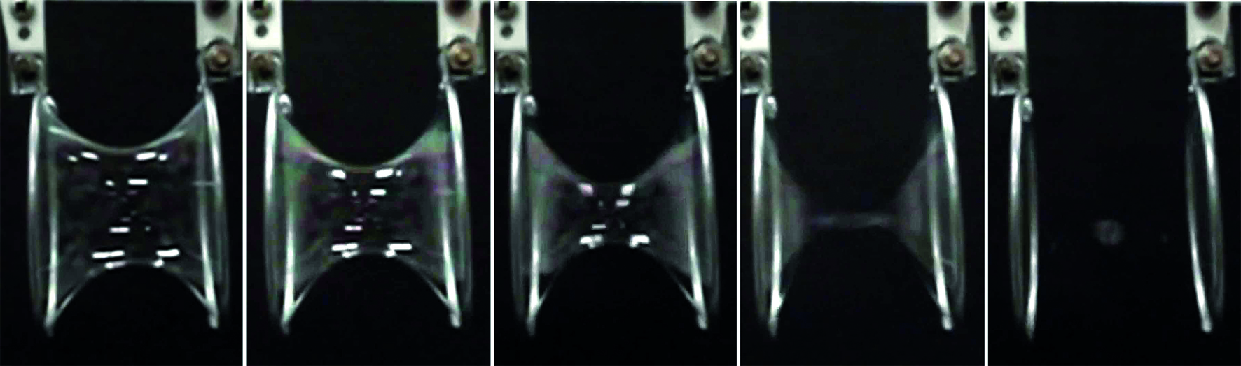
Consider a soap film between two parallel circles of diameter 1, at small distance. We obtain a catenoid as in the left picture of Figure 1. When the separation (distance) between the two circles is small, the catenoid is an area minimizing surface. However, as we separate the circles more and more, we will reach a first critical separation, after which the area of the catenoid will be greater than . Now the catenoidal soap films are no longer minimizers of the area (two flat disks joined with a thin neck would outperform them) but this does not cause any instability. Then, if we continue separating the circles, we reach a second critical separation, after which the soap film breaks into two disconnected disks, as shown in Figure 1.
All rights reserved.
What happens between the two critical separations? The answer is given by the notion of stable minimal surface: although these catenoids are not “absolute” minimizers of the area, they still have a lesser area than any small variation of them. And this is enough to stabilize them.
As the previous example shows, not only energy minimizers are found in nature. Also stable solutions, i.e., those outperforming any small perturbation of them, are of physical interest. However, for Plateau’s problem, as well as for several other important non-convex variational problems, fundamental questions that are well-understood in the case of minimizers remain completely open in the case of stable solutions. We next give a concrete example that will motivate some of our results described later.
A priori curvature bounds
The nowadays standard regularity theory for area minimizers – see (i) above – implies the following:
Let and be an area minimizing hypersurface in the unit ball . Then the curvatures of inside the half ball are bounded by dimensional constants.
It has long been conjectured3In the case this is Schoen’s conjecture (see [12 T. H. Colding and W. P. Minicozzi, II, A Course in Minimal Surfaces. Graduate Studies in Mathematics 121, American Mathematical Society, Providence, RI (2011) , Chapter 2]). that
Conjecture 2. Theorem 1 holds replacing “area minimizing hypersurface” by “stable minimal hypersurface”.
By a simple (though clever) scaling and compactness argument of White (see [44 B. White, Lecture notes in minimal surface theory. arXiv:1308.3325 (2013) ]), Conjecture 2 is equivalent to
Conjecture 3. Let and be a connected, complete, stable minimal hypersurface. Then is an hyperplane.
The previous conjectures have been proved only in the case (surfaces in ); the earliest proofs date from the 1970’s, see [12 T. H. Colding and W. P. Minicozzi, II, A Course in Minimal Surfaces. Graduate Studies in Mathematics 121, American Mathematical Society, Providence, RI (2011) ]. But, unfortunately, their beautiful and relatively short proofs are extremely specific to the case of minimal surfaces in : they cannot be extended to higher dimensions, nor even to other interface models in which are very similar to minimal surfaces.
2 Interfaces in phase transitions
The Allen–Cahn equation
Consider a binary fluid, i.e., a mixture containing two types of molecule: A and B (like oil and water). In many cases, these molecules have an energetic preference to be surrounded by others of their same kind. It undergoes phase separation into A-rich and B-rich regions.
Phase transition and phase separation phenomena – such as the previous one – are modelled by means of the scalar Ginzburg–Landau energy:
defined on scalar fields , where . Here is a so-called double-well potential with “wells” (i.e., minima) at . Typically one takes .
Scalar fields satisfying
for all are called critical points (in ) of . They solve the Allen–Cahn equation: . A critical point is called a minimizer (in ) if , for all .
Let us come back to the binary fluid example to see how the scalar fields encode A-rich and B-rich regions. The idea is to interpret , a number in the interval , as the relative density of molecules of type A at . In other words, means that belongs to a A-rich region while means that belongs to a B-rich region.
When the parameter is small the potential strongly penalizes intermediate states and the space essentially splits into two regions, (A-rich region) and (B-rich region), which are separated by an interface (mixture of both molecules). The interface is a “fat surface” of thickness . On the other hand, the Dirichlet term of the energy makes transitions between costly, so interfaces are energetically expensive.
The zero level set can be thought as the surface which best approximates the interface .
An important family of explicit solutions to the Allen–Cahn equation is given by
where and . Via a calibration argument [4 L. Ambrosio and X. Cabré, Entire solutions of semilinear elliptic equations in 𝐑3 and a conjecture of De Giorgi. J. Amer. Math. Soc.13, 725–739 (2000) ], one can see that are minimizers of in all of .
Connection with minimal surfaces
By the results in [10 L. A. Caffarelli and A. Córdoba, Uniform convergence of a singular perturbation problem. Comm. Pure Appl. Math.48, 1–12 (1995) , 30 L. Modica and S. Mortola, Un esempio di Γ--convergenza. Boll. Un. Mat. Ital. B (5)14, 285–299 (1977) ], if is a sequence of minimizers of , then the surfaces converge locally uniformly4In the sense of the Hausdorff distance and up to subsequences., as , towards area minimizing hypersurfaces.
It is then natural to ask if the surfaces inherit the regularity properties of the area minimizing hypersurfaces to which they converge. In other words:
Is smooth in dimensions , with robust estimates as ?
This delicate question is nowadays completely understood in the case of energy minimizers. Indeed, Savin established in 2009 the following celebrated result.
Assume that . Let be a minimizer of in with . Then is a hypersurface, with robust estimates as .
A “famous” consequence of Theorem 1 and scaling is that any minimizer of in all of must be either or of the form (2.1) with .
Combining Savin’s result with the recent estimates of Wang and Wei [42 K. Wang and J. Wei, Second order estimate on transition layers. Adv. Math.358, 106856, 85 (2019) ] we obtain:
Assume that . Let be a minimizer of in with . Then, the curvatures of the hypersurface are bounded by dimensional constants in .
Conjectures on stable solutions
As in the case of soap films, it is very natural to ask:
Does Theorem 5 hold when “minimizer” is replaced by “stable critical point” (i.e., minimizer among small perturbations)?
Like for minimal surfaces, thanks to the striking results from [42 K. Wang and J. Wei, Second order estimate on transition layers. Adv. Math.358, 106856, 85 (2019) ], the previous question can be reduced to the following long-standing
Conjecture 6. Assume that . Let be a stable critical point of in the whole space different from . Then must be of the form (2.1) with .
Even in the case of , Conjecture 6 is a very challenging and completely open problem (although the analogous result for minimal surfaces in is known, its very rigid proof does not generalize to stable critical points of ). The case of , which is already nontrivial, was proven by Ambrosio and Cabré [4 L. Ambrosio and X. Cabré, Entire solutions of semilinear elliptic equations in 𝐑3 and a conjecture of De Giorgi. J. Amer. Math. Soc.13, 725–739 (2000) ] in 2000.
Interestingly, Conjecture 6 is known to imply a famous 1979 conjecture of De Giorgi [16 E. De Giorgi, Convergence problems for functionals and operators. In Proceedings of the International Meeting on Recent Methods in Nonlinear Analysis (Rome, 1978), Pitagora, Bologna, 131–188 (1979) ]: for all (one dimension more than before) any solution of the Allen–Cahn equation in the whole space satisfying must be of the form (2.1), with and .
“Counterexamples” to Theorem 5 and Conjecture 6 for , and to De Giorgi’s conjecture for were obtained – via very delicate and involved constructions – in [17 M. del Pino, M. Kowalczyk and J. Wei, On De Giorgi’s conjecture in dimension N≥9. Ann. of Math. (2)174, 1485–1569 (2011) , 29 Y. Liu, K. Wang and J. Wei, Global minimizers of the Allen-Cahn equation in dimension n≥8. J. Math. Pures Appl. (9)108, 818–840 (2017) ].
The Peierls–Nabarro equation
Introduced in the early 1940’s in the context of crystal dislocations [33 R. Peierls, The size of a dislocation. Proc. Phys. Soc.52, 34–37 (1940) , 32 F. Nabarro, Dislocations in a simple cubic lattice. Proc. Phys. Soc.59, 256–272 (1947) ], the Peierls–Nabarro equation also models phase transitions with line-tension effects [1 G. Alberti, G. Bouchitté and P. Seppecher, Phase transition with the line-tension effect. Arch. Rational Mech. Anal.144, 1–46 (1998) ] and boundary vortices in thin magnetic films [27 M. Kurzke, Boundary vortices in thin magnetic films. Calc. Var. Partial Differential Equations26, 1–28 (2006) ]. It concerns the energy functional
As in the previous section, is a scalar field and is a double-well potential.
In this context a natural double-well potential is , and for this choice of an explicit family of solutions is given by
The two functionals and behave similarly, and there is an almost perfect parallel between their interface regularity theories. To start with, by [1 G. Alberti, G. Bouchitté and P. Seppecher, Phase transition with the line-tension effect. Arch. Rational Mech. Anal.144, 1–46 (1998) , 38 O. Savin and E. Valdinoci, Density estimates for a variational model driven by the Gagliardo norm. J. Math. Pures Appl. (9)101, 1–26 (2014) ], if is a sequence of minimizers of then the interfaces converge locally uniformly as towards area minimizing hypersurfaces, just as they do for .
In this context the analogue of Theorem 4 – i.e., a local estimate for in the case of energy minimizers – was obtained in [37 O. Savin, Rigidity of minimizers in nonlocal phase transitions. Anal. PDE11, 1881–1900 (2018) ], also by Savin, using similar techniques.
Given the parallel between and , it is conjectured that for all stable critical points of in the whole space must be of the form (2.2) with (in other words that the analogue of Conjecture 6 replacing by holds).
While Conjecture 6 (for ) remains completely open in dimensions , Figalli and the author [23 A. Figalli and J. Serra, On stable solutions for boundary reactions: a De Giorgi-type result in dimension 4+1. Invent. Math.219, 153–177 (2020) ] were able to establish it for in dimension .
Let be a stable critical point of in the whole space . Then must be of the form (2.2) with .
This result finally broke the parallel of known results for and , in favour of . Its proof exploits the “long-range interactions” from the term
borrowing ideas from a paper of Cinti, the author, and Valdinoci [11 E. Cinti, J. Serra and E. Valdinoci, Quantitative flatness results and BV-estimates for stable nonlocal minimal surfaces. J. Differential Geom.112, 447–504 (2019) ] on nonlocal minimal surfaces.
3 The obstacle problem and Stefan’s problem
Pushing an elastic membrane with an obstacle
Given some smooth domain , and , both smooth and satisfying , consider the convex minimization problem
For , one can think of as the equilibrium position of an elastic membrane whose boundary is held fixed while it is pushed from below by an obstacle (the hypograph of ).
The function can be shown to satisfy in . In the “model case” one obtains
In other words, the domain is split into two subdomains and and inside the first one we have . The unknown interface between the two subdomains, denoted , is called the free boundary. Since must satisfy (3.1) (in the sense of distributions) in , not only but also must vanish continuously on . In this “double constraint” (3.1) encodes the geometric information about the free boundary.
As an interesting fact, solutions of (3.1) minimize the following convex energy functional:
A potential theoretic motivation of the obstacle problem
Imagine a cloud made of a very large number of identical point charges in . They interact through the standard Coulomb potential, repelling each other. In absence of external forces the cloud would expand indefinitely, but inside some exterior potential the cloud will reach an equilibrium, occupying only a bounded region of the space. This motivates the introduction of the so-called (Frostman) equilibrium measure for Coulomb interactions with an external “field” (growing at infinity), defined as the unique probability measure on which minimizes
Denoting by the potential generated by , the equilibrium measure is compactly supported and uniquely characterized by the fact that there exists a constant such that in and on the support of . In other words solves the obstacle problem in the whole space with obstacle .
Ice melting in water
Dating back to the 19th century, Stefan’s problem [41 J. Stefan, Über einige Probleme der Theorie der Wärmeleitung. Wien. Ber.98, 473–484 (1889) ] aims to describe the temperature distribution in a homogeneous medium undergoing a phase change, typically a body of ice at zero degrees centigrade submerged in water.
Its most classical formulation is as follows: let be some bounded domain, and let denote the temperature of the water at the point at time . We assume that on the ice and in the water. The temperature satisfies the heat equation inside the water and the Stefan condition5The normal velocity of is proportional to the flux of heat (which is used to melt the ice). By Fourier’s law this flux is proportional to the gradient of temperature, hence . But, since on the moving interface we obtain on , from which Stefan’s condition follows. on the interface .
Baiocchi and Duvaut [5 C. Baiocchi, Free boundary problems in the theory of fluid flow through porous media. In Proceedings of the International Congress of Mathematicians (Vancouver, B. C., 1974), Vol. 2, 237–243 (1975) , 18 G. Duvaut, Résolution d’un problème de Stefan (fusion d’un bloc de glace à zéro degré). C. R. Acad. Sci. Paris Sér. A–B276, A1461–A1463 (1973) ] introduced the transformation and showed that the new scalar field satisfies6Near points that were inside the ice at initial time and for .
In addition, by definition of we have and
Interestingly, the evolution (3.4) is the gradient flow of the convex functional (3.2). Thanks to this convex structure, some basic questions such as existence and well-posedness of Stefan’s problem – which would be very non-obvious in the original formulation – can be shown via standard Functional Analysis methods.
Other motivations
Stefan’s and obstacle problems have other well-known applications in physics, biology, or financial mathematics. Some examples are: the dam problem, the Hele–Shaw flow, pricing of American options, quadrature domains, random matrices, etc.
Regularity of free boundaries: Main questions and difficulties
Any solution of (3.4) can be shown to be of class in space and in time. This regularity is optimal because the right hand side in (3.4) forces to be discontinuous across .
The most interesting regularity questions concern the free boundary:
Is the free boundary a smooth hypersurface, or may it have singularities?
If the singular set is nonempty, how “large” can it be?
Classical examples by Lévy and Schaeffer (some known from before the 1970’s) show that solutions of the obstacle problem with non-smooth free boundaries exist already in the smallest nontrivial dimension ; see [26 D. Kinderlehrer and L. Nirenberg, Regularity in free boundary problems. Ann. Scuola Norm. Sup. Pisa Cl. Sci. (4)4, 373–391 (1977) ]. Hence, any positive regularity result on the free boundary must be “conditional”.
It was not until 1977, with the groundbreaking paper of Caffarelli [8 L. A. Caffarelli, The regularity of free boundaries in higher dimensions. Acta Math.139, 155–184 (1977) ], that a regularity theory for the free boundaries of solutions of (3.4) was established. Since (3.1) is a particular case of (3.4) – that of constant in time solutions – Caffarelli’s results apply at the same time to both the obstacle problem and Stefan’s problem.
Caffarelli’s breakthrough
The approach of Caffarelli to the regularity of free boundaries of (3.4) – or of (3.1) – has some similarities with the regularity theory of area minimizing hypersurfaces described in Section 1. In Caffarelli’s regularity theory (as in minimal surfaces) blow-ups are very important actors. Informally speaking, one looks at the free boundary through a microscope, and then tries to infer its “macroscopic properties” from its “microscopic” ones.
For (3.4) the scaling of the problem suggests considering, for given and ,
It is easy to see that is again a solution of (3.4). Blow-ups are defined as accumulation points of as .
The main results from [8 L. A. Caffarelli, The regularity of free boundaries in higher dimensions. Acta Math.139, 155–184 (1977) ] (combined with [26 D. Kinderlehrer and L. Nirenberg, Regularity in free boundary problems. Ann. Scuola Norm. Sup. Pisa Cl. Sci. (4)4, 373–391 (1977) ], [9 L. A. Caffarelli, The obstacle problem revisited. J. Fourier Anal. Appl.4, 383–402 (1998) ] and [6 A. Blanchet, On the singular set of the parabolic obstacle problem. J. Differential Equations231, 656–672 (2006) ]) can be summarized as follows:
Let and be a solution of (3.4). For every belonging to the free boundary one of the following two alternatives holds:
as , for some ; and the free boundary is a (moving) analytic embedded -surface near .
as , for some nonnegative definite matrix with trace equal to ; and the free boundary has a singularity7For the evolutionary problem (3.4) singularities are associated to changes of topology of the ice . For instance, the ice may develop a very thin shrinking neck which eventually breaks into two pieces after producing a singular point. at .
Further known results on singular points
After the results of Caffarelli [8 L. A. Caffarelli, The regularity of free boundaries in higher dimensions. Acta Math.139, 155–184 (1977) ], a natural question is: what else can be said about singular points?
For the obstacle problem (3.1) in dimension , Sakai [34 M. Sakai, Regularity of a boundary having a Schwarz function. Acta Math.166, 263–297 (1991) , 35 M. Sakai, Regularity of free boundaries in two dimensions. Ann. Scuola Norm. Sup. Pisa Cl. Sci. (4)20, 323–339 (1993) ] used methods in complex analysis to give an extremely accurate description of the possible singularities. In particular, the results of Sakai imply that at every singular free boundary point of a solution of (3.1) in we have
with . This significantly improved the qualitative description of Theorem 8(b), which is equivalent to , and entailed some interesting consequences. Unfortunately, Sakai’s complex analysis methods cannot work in higher dimensions, nor for Stefan’s problem (not even for ). Thus, improving Caffarelli’s result for (3.1) in dimensions required new ideas.
Understanding singularities better
The first new result in this direction for was established by Colombo, Spolaor, and Velichkov in 2017 [13 M. Colombo, L. Spolaor and B. Velichkov, A logarithmic epiperimetric inequality for the obstacle problem. Geom. Funct. Anal.28, 1029–1061 (2018) ]. By improving and refining the methods of Weiss [43 G. S. Weiss, A homogeneity improvement approach to the obstacle problem. Invent. Math.138, 23–50 (1999) ], they proved that at every singular point, the expansion (3.6) holds with explicit logarithmic modulus of continuity , where . Independently and with different methods, Figalli and the author proved in [22 A. Figalli and J. Serra, On the fine structure of the free boundary for the classical obstacle problem. Invent. Math.215, 311–366 (2019) ] the following:
Let be a solution of the obstacle problem (3.1) with . For all singular points outside some “anomalous” set of Hausdorff dimension , (3.6) holds with . Moreover, there exist examples in of isolated singular points for which as for all .
The previous theorem suggests, for one thing, that we may be able to give a very precise quantitative description of most singularities. However, the existence – already in – of singular points for which for all tells us that we cannot hope for some analytic structure of singularities as in Sakai’s result for : in higher dimensions some singularities may be very complicated.
Another insightful result from [22 A. Figalli and J. Serra, On the fine structure of the free boundary for the classical obstacle problem. Invent. Math.215, 311–366 (2019) ] is that, for all singular points outside some -dimensional set we have, after rotation, the improved expansion , where is some quadratic polynomial satisfying . This invites us to investigate higher order expansions that hold at most singular points (although proving this turned out to be quite a delicate task, and the tools needed to complete it were only developed later in [20 A. Figalli, X. Ros-Oton and J. Serra, Generic regularity of free boundaries for the obstacle problem. Publ. Math. Inst. Hautes Études Sci.132, 181–292 (2020) ]).
It is interesting to notice that the methods introduced in [22 A. Figalli and J. Serra, On the fine structure of the free boundary for the classical obstacle problem. Invent. Math.215, 311–366 (2019) ] for the obstacle problem are closely connected with Almgren’s regularity theory [3 F. J. Almgren, Jr., Almgren’s big regularity paper. World Scientific Monograph Series in Mathematics 1, World Scientific Publishing Co., Inc., River Edge, NJ (2000) ] for mass minimizing -surfaces in with . In particular, Almgren’s frequency formula plays an important (and unexpected) role.
The size of the singular set
An important consequence of Theorem 8 is that, in both the obstacle and Stefan’s problems, the singular sets enjoy spatial -regularity, in the sense that they can be covered by -manifolds of class (see [9 L. A. Caffarelli, The obstacle problem revisited. J. Fourier Anal. Appl.4, 383–402 (1998) , 6 A. Blanchet, On the singular set of the parabolic obstacle problem. J. Differential Equations231, 656–672 (2006) ]). Note, however, that this is not a very useful piece of information on the size of the singular set, since the regular part of the free boundary is also -dimensional and thus, a priori, the singular part could be as large as the regular one.
As explained above, Theorem 8 applies at the same time to both the obstacle problem and Stefan’s problem, since (3.1) is a particular case of (3.4). However, when we seek to obtain improved bounds on the size of their singular sets, the two problems need to be treated in completely different ways. On the one hand, in Stefan problem it is natural to try to exploit (3.5) – which was not used in Caffarelli’s theory – and to ask if the free boundary is free of singularities most of the time. On the other hand, for the stationary problem (3.1), the previous evolutionary point of view makes no sense. In the absence of time, the only thing one can hope to prove is that for “generic” boundary values, solutions of (3.1) do not have singular points. This is actually something that has been expected to be true since the 1970’s [39 D. G. Schaeffer, An example of generic regularity for a non-linear elliptic equation. Arch. Rational Mech. Anal.57, 134–141 (1975) ]:
Conjecture 10 (Schaeffer, 1974). Generically, solutions of the obstacle problem have smooth free boundaries.
Until recently Conjecture 10 was only known to hold in the plane (see [31 R. Monneau, On the number of singularities for the obstacle problem in two dimensions. J. Geom. Anal.13, 359–389 (2003) ]).
Generic regularity for the obstacle problem
Building on the methods initiated in [22 A. Figalli and J. Serra, On the fine structure of the free boundary for the classical obstacle problem. Invent. Math.215, 311–366 (2019) ] we were recently able to obtain a positive answer to Schaeffer’s conjecture in low dimensions:
Conjecture 10 holds in and .
Our strategy towards this theorem is reminiscent of Sard’s theorem in analysis. By adding to the boundary values we produce a monotone 1-parameter family of solutions. We then prove that the set of “singular values” of has measure zero by improving the order of approximation of certain polynomial expansions at most singular points. This is a long and delicate proof because the singular sets need to be split into several different strata, and in each of them the corresponding singular values have measure zero for very different reasons.
The singular set in Stefan’s problem
As said above, in order to investigate the size of the singular set in Stefan’s problem, we will use (3.5). In particular, from now on solutions will never be stationary.
Fix and let be a solution of (3.4)–(3.5). It will be useful to define the spatial and time projections and .
Let us denote by the set of all singular free boundary points of .
Caffarelli’s regularity theory implies (see [9 L. A. Caffarelli, The obstacle problem revisited. J. Fourier Anal. Appl.4, 383–402 (1998) , 6 A. Blanchet, On the singular set of the parabolic obstacle problem. J. Differential Equations231, 656–672 (2006) ]) that every “time slice” of can be locally covered by -manifolds of class . This may not seem like a very strong piece of information, since the regular part of the free boundary is also -dimensional. However, it is not difficult to construct solutions of (3.4)–(3.5) with rotational symmetry such that for countably many times the time slice contains some -sphere .
The previous examples show that even for countably many times, the singular set can have positive -dimensional measure. At those times, the singular set is as large as the regular part of the free boundary. Still, inspection of explicit examples suggests that should be smaller in some sense than the regular part of the free boundary, perhaps as a subset of the “space-time” .
Until recently, the best results available in this direction, such as [28 E. Lindgren and R. Monneau, Pointwise regularity of the free boundary for the parabolic obstacle problem. Calc. Var. Partial Differential Equations54, 299–347 (2015) ], could not even rule out being -dimensional for every time !
In the forthcoming article [21 A. Figalli, X. Ros-Oton and J. Serra, The singular set in Stefan’s problem. Forthcoming preprint. ], we are able to prove a much stronger result, which gives a precise structure and sharp dimensional bounds on the singular set of Stefan’s problem.
There exist such that the following holds:
, where denotes the parabolic Hausdorff dimension;8For and , we say that if, for all , can be covered by countably many parabolic cylinders making arbitrarily small. This notion of Hausdorff dimension is well-adapted to the parabolic scaling under which (3.4) is invariant.
can be covered by countably many -manifolds;
has zero Hausdorff dimension.
This is a very precise result. Recall that in radial examples the singular set can contain some -sphere countably many times. Such spheres would be covered by the set in Theorem 12. Now, we cannot prove that in general is countable as it is in such examples, but we do show that it is a 0-dimensional set (and Hausdorff dimension cannot distinguish between countable and 0-dimensional sets, so the result is sharp in this sense). However, the complement of inside is a set of “bad” singular points. These “bad” points do not a priori enjoy any extra spatial regularity, but in exchange they are lower-dimensional: their parabolic Hausdorff dimension is bounded by . This bound is also optimal, as can be shown by considering any radial solution in with a singular point at .
An important consequence of Theorem 12 is the following:
Corollary 13 ([21 A. Figalli, X. Ros-Oton and J. Serra, The singular set in Stefan’s problem. Forthcoming preprint. ]). The set of singular times for Stefan’s problem in has Hausdorff dimension at most . In particular, it has measure zero.
Also, Theorem 12 implies that in the set of singular times for Stefan’s problem has zero Hausdorff dimension (prior to our results it was not even known that in the set of singular times had measure zero).
- 1
-dimensional surface.
- 2
This is an intentionally imprecise notion: more rigorously, can be the boundary of a set of minimal perimeter, or a mass minimizing integer rectifiable current.
- 3
In the case this is Schoen’s conjecture (see [12 T. H. Colding and W. P. Minicozzi, II, A Course in Minimal Surfaces. Graduate Studies in Mathematics 121, American Mathematical Society, Providence, RI (2011) , Chapter 2]).
- 4
In the sense of the Hausdorff distance and up to subsequences.
- 5
The normal velocity of is proportional to the flux of heat (which is used to melt the ice). By Fourier’s law this flux is proportional to the gradient of temperature, hence . But, since on the moving interface we obtain on , from which Stefan’s condition follows.
- 6
Near points that were inside the ice at initial time and for .
- 7
For the evolutionary problem (3.4) singularities are associated to changes of topology of the ice . For instance, the ice may develop a very thin shrinking neck which eventually breaks into two pieces after producing a singular point.
- 8
For and , we say that if, for all , can be covered by countably many parabolic cylinders making arbitrarily small. This notion of Hausdorff dimension is well-adapted to the parabolic scaling under which (3.4) is invariant.
References
- G. Alberti, G. Bouchitté and P. Seppecher, Phase transition with the line-tension effect. Arch. Rational Mech. Anal.144, 1–46 (1998)
- F. J. Almgren, Jr., Some interior regularity theorems for minimal surfaces and an extension of Bernstein’s theorem. Ann. of Math. (2)84, 277–292 (1966)
- F. J. Almgren, Jr., Almgren’s big regularity paper. World Scientific Monograph Series in Mathematics 1, World Scientific Publishing Co., Inc., River Edge, NJ (2000)
- L. Ambrosio and X. Cabré, Entire solutions of semilinear elliptic equations in 𝐑3 and a conjecture of De Giorgi. J. Amer. Math. Soc.13, 725–739 (2000)
- C. Baiocchi, Free boundary problems in the theory of fluid flow through porous media. In Proceedings of the International Congress of Mathematicians (Vancouver, B. C., 1974), Vol. 2, 237–243 (1975)
- A. Blanchet, On the singular set of the parabolic obstacle problem. J. Differential Equations231, 656–672 (2006)
- E. Bombieri, E. De Giorgi and E. Giusti, Minimal cones and the Bernstein problem. Invent. Math.7, 243–268 (1969)
- L. A. Caffarelli, The regularity of free boundaries in higher dimensions. Acta Math.139, 155–184 (1977)
- L. A. Caffarelli, The obstacle problem revisited. J. Fourier Anal. Appl.4, 383–402 (1998)
- L. A. Caffarelli and A. Córdoba, Uniform convergence of a singular perturbation problem. Comm. Pure Appl. Math.48, 1–12 (1995)
- E. Cinti, J. Serra and E. Valdinoci, Quantitative flatness results and BV-estimates for stable nonlocal minimal surfaces. J. Differential Geom.112, 447–504 (2019)
- T. H. Colding and W. P. Minicozzi, II, A Course in Minimal Surfaces. Graduate Studies in Mathematics 121, American Mathematical Society, Providence, RI (2011)
- M. Colombo, L. Spolaor and B. Velichkov, A logarithmic epiperimetric inequality for the obstacle problem. Geom. Funct. Anal.28, 1029–1061 (2018)
- E. De Giorgi, Frontiere orientate di misura minima. Seminario di Matematica della Scuola Normale Superiore di Pisa, 1960–61, Editrice Tecnico Scientifica, Pisa (1961)
- E. De Giorgi, Una estensione del teorema di Bernstein. Ann. Scuola Norm. Sup. Pisa Cl. Sci. (3)19, 79–85 (1965)
- E. De Giorgi, Convergence problems for functionals and operators. In Proceedings of the International Meeting on Recent Methods in Nonlinear Analysis (Rome, 1978), Pitagora, Bologna, 131–188 (1979)
- M. del Pino, M. Kowalczyk and J. Wei, On De Giorgi’s conjecture in dimension N≥9. Ann. of Math. (2)174, 1485–1569 (2011)
- G. Duvaut, Résolution d’un problème de Stefan (fusion d’un bloc de glace à zéro degré). C. R. Acad. Sci. Paris Sér. A–B276, A1461–A1463 (1973)
- H. Federer, The singular sets of area minimizing rectifiable currents with codimension one and of area minimizing flat chains modulo two with arbitrary codimension. Bull. Amer. Math. Soc.76, 767–771 (1970)
- A. Figalli, X. Ros-Oton and J. Serra, Generic regularity of free boundaries for the obstacle problem. Publ. Math. Inst. Hautes Études Sci.132, 181–292 (2020)
- A. Figalli, X. Ros-Oton and J. Serra, The singular set in Stefan’s problem. Forthcoming preprint.
- A. Figalli and J. Serra, On the fine structure of the free boundary for the classical obstacle problem. Invent. Math.215, 311–366 (2019)
- A. Figalli and J. Serra, On stable solutions for boundary reactions: a De Giorgi-type result in dimension 4+1. Invent. Math.219, 153–177 (2020)
- W. H. Fleming, On the oriented Plateau problem. Rend. Circ. Mat. Palermo (2)11, 69–90 (1962)
- M. Ito and T. Sato, In situ observation of a soap-film catenoid – a simple educational physics experiment. European J. Phys.31, 357–365 (2010)
- D. Kinderlehrer and L. Nirenberg, Regularity in free boundary problems. Ann. Scuola Norm. Sup. Pisa Cl. Sci. (4)4, 373–391 (1977)
- M. Kurzke, Boundary vortices in thin magnetic films. Calc. Var. Partial Differential Equations26, 1–28 (2006)
- E. Lindgren and R. Monneau, Pointwise regularity of the free boundary for the parabolic obstacle problem. Calc. Var. Partial Differential Equations54, 299–347 (2015)
- Y. Liu, K. Wang and J. Wei, Global minimizers of the Allen-Cahn equation in dimension n≥8. J. Math. Pures Appl. (9)108, 818–840 (2017)
- L. Modica and S. Mortola, Un esempio di Γ--convergenza. Boll. Un. Mat. Ital. B (5)14, 285–299 (1977)
- R. Monneau, On the number of singularities for the obstacle problem in two dimensions. J. Geom. Anal.13, 359–389 (2003)
- F. Nabarro, Dislocations in a simple cubic lattice. Proc. Phys. Soc.59, 256–272 (1947)
- R. Peierls, The size of a dislocation. Proc. Phys. Soc.52, 34–37 (1940)
- M. Sakai, Regularity of a boundary having a Schwarz function. Acta Math.166, 263–297 (1991)
- M. Sakai, Regularity of free boundaries in two dimensions. Ann. Scuola Norm. Sup. Pisa Cl. Sci. (4)20, 323–339 (1993)
- O. Savin, Regularity of flat level sets in phase transitions. Ann. of Math. (2)169, 41–78 (2009)
- O. Savin, Rigidity of minimizers in nonlocal phase transitions. Anal. PDE11, 1881–1900 (2018)
- O. Savin and E. Valdinoci, Density estimates for a variational model driven by the Gagliardo norm. J. Math. Pures Appl. (9)101, 1–26 (2014)
- D. G. Schaeffer, An example of generic regularity for a non-linear elliptic equation. Arch. Rational Mech. Anal.57, 134–141 (1975)
- J. Simons, Minimal varieties in riemannian manifolds. Ann. of Math. (2)88, 62–105 (1968)
- J. Stefan, Über einige Probleme der Theorie der Wärmeleitung. Wien. Ber.98, 473–484 (1889)
- K. Wang and J. Wei, Second order estimate on transition layers. Adv. Math.358, 106856, 85 (2019)
- G. S. Weiss, A homogeneity improvement approach to the obstacle problem. Invent. Math.138, 23–50 (1999)
- B. White, Lecture notes in minimal surface theory. arXiv:1308.3325 (2013)
Cite this article
Joaquim Serra, The geometric structure of interfaces and free boundaries. Eur. Math. Soc. Mag. 120 (2021), pp. 8–15
DOI 10.4171/MAG/17